Renewable Modelling · Grid-Side Scan & Series Compensation

The Grid-Side Impedance Scan for SSCI in EMTP®

Series compensation, post-fault topology and reading R(f) / X(f)

A grid-side impedance scan characterises the passive network seen from the wind-park interface after a fault has been cleared. The setting is a small grid with a series-compensated line — the classic DFIG SSCI hazard, because the series capacitor offsets the line inductance and creates a resonance below the fundamental frequency. The risk is usually made by the post-fault topology: a fault opens breakers and leaves the wind park on the remaining compensated corridor, changing the network it sees, so that remaining topology can hold a subsynchronous resonance that must be identified before the turbine-side impedance is added. Because that network is linear and passive, its impedance comes straight from a fast phasor-domain scan. What follows sets out the series-compensation resonance, why the post-fault network defines the study, the phasor-versus-time-domain choice, and how to read the resulting R(f) and X(f) curves.

Reading time ≈ 18 min · series compensation, post-fault topology & the grid scan

A grid-side impedance scan characterises the passive network seen from the wind-park interface after a fault has been cleared. The setting is a small grid with a series-compensated line — the textbook DFIG SSCI hazard — where the network left after clearing can hold a subsynchronous resonance. What follows builds the grid side of the combined impedance scan: how the post-fault network defines what is scanned, why the grid is characterised first, and how to read its \(R(f)\) and \(X(f)\) signature before the turbine impedance is added.

Abbreviations used on this page

SSCISub-synchronous control interaction

SSRSub-synchronous resonance

DFIGDoubly-fed induction generator

\(f_{er}\)Electrical resonant frequency

\(f_0\)Fundamental frequency

\(X_C,X_L\)Capacitor, line reactance

\(k\)Degree of series compensation

\(Z(f)\)Frequency-dependent impedance

\(R,X\)Resistance, reactance

TDTime domain

EMTElectromagnetic transient

EMTP®Electromagnetic Transients Program

Key idea

A series-compensated line is the classic DFIG SSCI hazard: the series capacitor offsets the line inductance and creates an electrical resonance \(f_{er}=f_0\sqrt{X_C/X_L}\) below the fundamental — a subsynchronous mode the network can support.
The risk is usually made by the post-fault topology: a fault opens breakers and leaves the wind park on the remaining compensated corridor, so the impedance it sees, the resonance and the damping all change. That post-fault network is what gets scanned.
The grid is scanned first. Because the remaining network is linear and passive, its impedance comes from a fast phasor-domain scan; a converter-rich side instead needs a time-domain scan.
The grid-side \(R(f)\) and \(X(f)\) curves show a sharp peak and a reactance zero-crossing at the subsynchronous resonance — the candidate frequency. The grid scan alone does not prove instability; it must be combined with the turbine impedance.

Key terms used on this page

01Series compensation

A series capacitor in a line that offsets its inductance to raise transfer capacity.

02Electrical resonant frequency

\(f_{er}\), where the capacitor and line reactances cancel; below fundamental for partial compensation.

03Degree of compensation

\(k=X_C/X_L\); the fraction of line reactance offset by the capacitor.

04SSCI

Sub-synchronous control interaction: instability between converter control and a network mode.

05Post-fault topology

The network configuration left after breakers clear a fault; it defines what is screened.

06Thévenin impedance

The equivalent network impedance seen by the plant from the interface; changes with topology.

07Phasor-domain scan

A frequency-domain impedance scan, valid and fast for a linear passive network.

08Time-domain scan

A perturbation-based impedance scan needed when the side is nonlinear or converter-controlled.

09Scan point

The interface bus where the impedance probe \(Z(f)\) is connected.

10Reactance zero-crossing

The frequency where \(X(f)\) changes sign — the resonance candidate.

11Subsynchronous range

Frequencies below the fundamental, where SSCI typically occurs; the scan window.

12Grid signature

The network’s \(R(f)\) and \(X(f)\) curves, to be combined with the turbine impedance.

Section 1

From method to setup

A grid-side impedance scan starts by defining the network condition to be studied. For SSCI screening, that condition is often the post-fault topology rather than the normal pre-fault network. The network you scan is not a given but something defined by an event, so before any scanning it is worth being clear about what system is under study and why it is risky.

Section 2

A small grid with a series-compensated line

The system studied here is a small grid with a series-compensated line. That detail is not incidental — series compensation is one of the classic situations in which DFIG-based wind plants can get into trouble. A series capacitor is installed to offset part of the line’s inductive reactance and so increase its power-transfer capability, but in doing so it changes the line reactance and introduces a resonant frequency below the fundamental. The network can then naturally support an oscillation at a subsynchronous frequency, and if the DFIG control interacts badly with that frequency, SSCI can appear.

Section 3

How series compensation creates a subsynchronous resonance

Sub-synchronous control interaction (SSCI) is an oscillatory interaction between converter controls and the network at frequencies below the fundamental. It is one form of the broader sub-synchronous resonance (SSR) family; the distinction is that SSCI specifically involves the converter and its control, rather than a purely electromechanical (shaft-torsional) resonance. The mechanism that sets the stage here is a series resonance: the series capacitor reduces the net inductive reactance of the corridor, so at a particular frequency the capacitor reactance and the line inductive reactance cancel, and because the capacitor only offsets part of the inductance, that resonance sits below the fundamental:

\[ f_{er} = f_0\sqrt{\frac{X_C}{X_L}} = f_0\sqrt{k}, \qquad k = \frac{X_C}{X_L} \lt 1 \ \Rightarrow\ f_{er} \lt f_0 \]

\(f_{er}\): electrical (series) resonant frequency
\(f_0\): fundamental frequency (50 or 60 Hz)
\(X_C,X_L\): capacitor and line reactances (at \(f_0\))
\(k=X_C/X_L\): degree of compensation (typically a fraction)

For partial compensation \(k\lt 1\), so \(f_{er}\) is subsynchronous — the network has a natural electrical mode below the fundamental. In the example scanned below, that mode sits near 14–15 Hz. Because the inductive and capacitive reactances cancel there, this is exactly the frequency at which the \(X(f)\) curve later crosses zero; it is also the mode a DFIG’s fast control can interact with. This 14–15 Hz value is specific to this example network, its compensation level and topology — not a general series-compensation frequency.

Section 4

Why DFIG plus series compensation is a classic concern

The hazard comes from pairing two things. A DFIG has its stator connected directly to the grid, with fast rotor-side converter control and a quick electrical and control response. A series-compensated line brings capacitive compensation into the transmission path and, with it, a subsynchronous resonance point. Put a converter-controlled machine onto a network that has a natural subsynchronous mode and you have exactly the environment in which SSCI can grow — the converter’s control, reacting at subsynchronous frequencies, can feed energy into the network resonance instead of damping it. Series compensation on its own only creates a subsynchronous resonance frequency, though; whether that becomes unstable depends on the combined grid and turbine impedance, the damping and the converter-control response.

Section 5

The post-fault topology defines the study

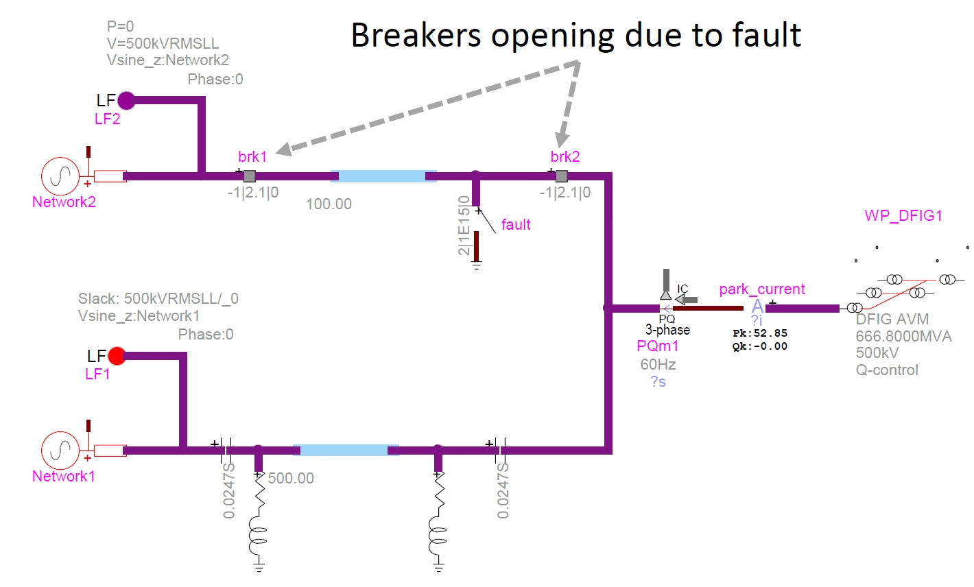
Here is the subtle, practical point. The risky network is often not the normal one but the one left after a disturbance. A fault occurs on one line; the breakers open and isolate the faulted path; and the wind park is then left connected through the remaining compensated corridor. After that switching, the Thévenin impedance the DFIG sees is different — the system strength changes, the resonant frequency shifts, and the damping changes. So SSCI is often not about the fault itself but about the post-fault configuration, which means the breaker action is not just a protection detail: it defines the system you are actually scanning. A different post-fault state gives a different resonance, so the scanned configuration must match the actual protection-cleared topology:

Match the scan to the protection-cleared topology

Breaker status
Line outages
Compensation level
Transformer status
Switched reactors and capacitors

Post-fault network single-line diagram: two grid infeeds (Grid A and Grid B) feed a substation bus; the faulted line is cleared with its breakers open and isolated, while the DFIG wind park stays connected through the series-compensated corridor that remains in service — the configuration screened for SSCI. — Figure 1 — Post-fault topology after breaker opening: the faulted path is isolated and the DFIG wind park remains connected through the series-compensated corridor. This is the passive network scanned for SSCI resonance.

Section 6

Scan the grid first

With the post-fault network defined, the workflow scans the grid first — the turbine is not yet included — because the grid is passive and linear enough to produce a clean frequency-domain impedance signature before the active turbine model is introduced. The scan is taken from the selected interface bus, looking outward into the external grid: an impedance probe returns the grid-side \(R(f)\) and \(X(f)\). Throughout, this grid-side impedance — equivalently the network or Thévenin impedance seen looking outward from the interface bus — is written \(Z_{grid}(f)=R(f)+jX(f)\). The logic is to characterise the network by itself, get its clean signature, and only then combine it with the turbine.

Section 7

Phasor-domain scan for a linear grid

Because the remaining network is linear and passive — lines, transformers, capacitors, reactors and resistances — it has a well-defined frequency response, so its impedance can be obtained directly in the phasor (frequency) domain. No time-domain perturbation is needed, which makes the grid scan very fast, essentially instantaneous. That is not true of every side, though:

Table 1 — Which scan suits which side.
Scan Type	Suitable Side	Why
Phasor / frequency domain	Linear, passive grid (lines, transformers, capacitors, reactors)	Well-defined frequency response; fast, near-instant
Time domain (perturbation)	Converter-rich / nonlinear side (wind turbines, VSC-HVDC)	Effective impedance depends on control and operating point, not just RLC

So a pure phasor-domain scan is enough for the passive grid, made of lines, transformers, capacitors, reactors and resistances. A converter-rich side cannot be treated the same way: its effective impedance depends on the controls, the limiters, the PLL behaviour and the operating point rather than on passive RLC physics, so it needs the time-domain scan.

Section 8

Reading the grid-side scan

The grid-side scan returns the network resistance and reactance versus frequency — the actual signature of the network seen by the turbine. Here \(R(f)\) represents the damping or loss in the scanned network, while \(X(f)\) shows whether the network appears inductive or capacitive at each frequency:

\[ Z_{grid}(f) = R_{grid}(f) + jX_{grid}(f), \qquad X_{grid}(f_{er}) = 0 \]

\(Z_{grid}(f)\): grid-side impedance from the scan
\(R_{grid},X_{grid}\): network resistance and reactance versus frequency
\(f_{er}\): the resonant frequency, where the reactance crosses zero

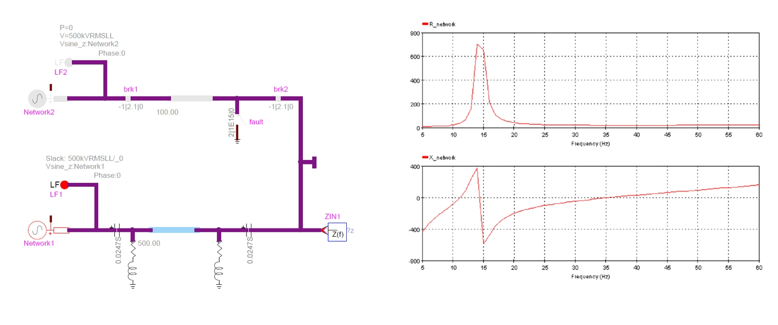
At the resonance the inductive and capacitive parts cancel, so \(X_{grid}\) crosses zero while \(R_{grid}\) shows a sharp peak nearby — the network telling you where it is naturally ready to oscillate. This resistance peak is the passive grid-side response, though: it does not by itself indicate negative damping, which appears only once the turbine/converter impedance is combined with this grid signature.

Grid-side impedance scan: the network resistance R_grid(f) shows a sharp peak near the subsynchronous resonance at about 14.5 Hz, while the reactance X_grid(f) changes sign and crosses zero at the same frequency, marking the resonant frequency f_er. — Figure 2 — The grid-side signature: \(R_{grid}(f)\) peaking and \(X_{grid}(f)\) crossing zero at the subsynchronous resonance, identifying the candidate frequency the network can support. A grid-side resonance is a candidate frequency for investigation, not a failed stability result.

Table 2 — Reading the two grid-side plots.
Plot	What It Shows	Signature at \(f_{er}\)
\(R_{grid}(f)\)	Network resistance versus frequency	A sharp peak near the resonance
\(X_{grid}(f)\)	Network reactance versus frequency	Sign change — a zero crossing (the resonance)

For a normal uncompensated network the reactance is mostly inductive over this range; the series capacitor is what lets the reactance reach zero, so the zero crossing is the direct fingerprint of the compensation. A zero crossing of \(X(f)\) indicates where the passive network changes from capacitive to inductive behaviour — not where instability is proven.

Section 9

Why scan from about 5 Hz to the fundamental

The scan window is chosen to match the physics. The fundamental is 50 or 60 Hz, and SSCI is a subsynchronous phenomenon — the suspicious interaction sits below the fundamental — so a window from roughly 5 Hz up to the fundamental covers the physically relevant region. This is deliberately not a search for switching harmonics, which live above the fundamental; it is a search for a control–electrical resonance below it, which is where the series-compensation mode and the converter interaction meet.

Section 10

What the grid scan does not yet tell you

It is important to be clear about the limits of this step. The grid scan alone does not prove instability; it only tells you the network has a resonant feature. To decide instability you still need the turbine-side impedance scan, and then the combination of both — because a grid resonance may be perfectly harmless if the turbine contributes positive damping there. So the natural next step is to compare the turbine-side impedance against this grid signature, and apply the zero-reactance, negative-resistance criterion to the total. Put plainly: a grid-side zero crossing is a location to investigate, not a failed stability result — the grid scan identifies the resonant frequency, and the damping assessment comes later, once the turbine-side impedance is added.

Half the picture

The grid scan finds where the network can oscillate. Whether that oscillation grows depends on the turbine: only the combined impedance, with its total resistance, decides damping.

Section 11

Why this is efficient

Because the phasor-domain grid scan takes essentially no time, it is a powerful screening tool in its own right. Different breaker configurations, compensation levels, post-fault topologies and line outages can each be scanned in moments, and the shift in the network resonance read off immediately — all before the turbine is even brought into the picture. So the grid scan lets you map the envelope of risky network conditions quickly, and reserve the heavier turbine and combined analysis for the configurations that actually show a worrying resonance.

Section 12

Key points

The post-fault compensated network, scanned in the phasor domain

The post-fault topology defines the scan: the breaker action that isolates the faulted line, not the fault itself, sets the network the wind park sees.
Series compensation can create a subsynchronous resonance \(f_{er}=f_0\sqrt{X_C/X_L}\) below the fundamental; whether it turns unstable depends on the combined impedance.
Because the grid is linear and passive, it can be scanned in the phasor domain — fast — whereas a converter-rich side needs a time-domain scan.
Reading \(R(f)\) and \(X(f)\), the \(X(f)=0\) crossing identifies the resonance candidate (with a sharp resistance peak nearby).
The grid scan alone does not prove instability: it must be combined with the turbine-side impedance and the zero-reactance, negative-resistance criterion applied to the total.

References

EMTP® Documentation and Application Notes. Powersys / EMTP®.

Built on EMTP® · Expert spotlight

Henry Gras

Chief Operating Officer, PGSTech · Montréal, Canada

Henry Gras delivers the EMTP® University course “EMT Simulation and Analysis of Large-Scale Power Systems with Renewables” and works daily with the tool this article is written around.

Henry is based in Montréal, where he is Chief Operating Officer of PGSTech, the company responsible for EMTP® engineering services, commercialisation and continuing software development. He holds a master’s degree from Polytechnique Montréal, where he worked on electrical-machine research, and previously completed an engineering degree at École Centrale de Lyon in France.

Readers who want a structured programme on EMT simulation of large-scale power systems with renewables will find his EMTP® University course an excellent next step.

Henry’s technical expertise covers electromagnetic transient simulation, renewable-energy integration, power-system modelling, electrical machines, protection and specialist transient studies including TRV, transformer energisation, ferroresonance, insulation coordination and power quality.

Part 27 Reading now

The Grid-Side Impedance Scan for SSCI

The grid-side scan under series compensation and post-fault topology, and reading R(f) and X(f).

Series progress 27 of 30

Part 28

The Turbine-Side Scan and SSCI Verification

Perturbation extraction, the combined scan and time-domain confirmation of the SSCI result.