Renewable Modelling · PV Cell Source Model

The PV Cell Source Model in EMTP®

Single-diode equivalent circuit, I-V/P-V curves and datasheet parameters

The dc source behind a PV inverter is not a fixed voltage source. A PV module is a nonlinear source whose terminal current depends on voltage, irradiance, temperature and internal cell parameters, captured by a single-diode equivalent circuit. That model reproduces the module’s I-V and P-V curves — including the maximum power point — which is exactly why the inverter extracts more or less power by moving the dc operating voltage. The single-diode model links the physical PV cell, the I-V/P-V curves and the MPPT operating point the inverter uses; the equivalent circuit and its current equation, the datasheet-based parameters and the connection to MPPT control follow below.

Reading time ≈ 18 min · single-diode model, I-V/P-V & datasheet parameters

The dc power a PV inverter delivers has to come from somewhere, and it comes from the PV array — which is not a fixed dc source but a nonlinear one, whose output depends on its terminal voltage, the irradiance and the temperature. A note on scale, because the terms are often mixed: a cell is the basic semiconductor device; a module (or panel) is a set of cells connected in series and parallel; and an array is the plant-level combination of modules and strings. The same single-diode model describes all three, scaled up. This page is about that electrical source model — the single-diode PV cell — and why its characteristic curve is the key to how an inverter chooses how much power to draw. It follows on from the PV park model.

Abbreviations used on this page

PVPhotovoltaic

MPPMaximum power point

MPPTMaximum-power-point tracking

STCStandard test conditions

\(I_{ph}\)Photocurrent (light-generated)

\(R_s,R_p\)Series, parallel (shunt) resistance

\(V_{oc}\)Open-circuit voltage

\(I_{sc}\)Short-circuit current

\(G\)Irradiance (W/m²)

\(N_s\)Cells in series per module

\(V_T\)Thermal voltage \(kT/q\)

EMTP®Electromagnetic Transients Program

Key idea

A PV module is modelled with a single-diode equivalent circuit — a photocurrent source in parallel with a diode and a shunt resistance \(R_p\), plus a series resistance \(R_s\) — not as a fixed ideal source.
Its output current depends on the terminal voltage, so the module has characteristic I–V and P–V curves with a maximum power point. Because \(P=V I\) and \(I\) itself depends on \(V\), changing the dc voltage moves the operating point and changes the extracted power — the basis of MPPT.
The diode makes the relation nonlinear and exponential in voltage; the photocurrent scales with irradiance and shifts with temperature, so the curve is not fixed but moves with the weather.
The parameters are derived from standard datasheet quantities (\(P_{max}\), \(V_{oc}\), \(I_{sc}\), the values at the MPP, the temperature coefficients and \(N_s\)) at standard test conditions, or taken from a module database — no lab tests needed.

Key terms used on this page

01Single-diode model

The standard PV equivalent circuit: photocurrent source, diode, shunt and series resistance.

02Photocurrent

The light-generated current \(I_{ph}\); the source part of the model, scaling with irradiance.

03Diode

Represents the cell p–n junction; its exponential current makes the model nonlinear.

04Series resistance \(R_s\)

Resistive losses in the current path; affects the fill factor and the high-current slope.

05Shunt resistance \(R_p\)

The shunt/parallel leakage resistance; a higher \(R_p\) means less leakage and a better low-voltage I–V slope.

06I–V curve

Output current versus terminal voltage; nearly flat then collapsing near open circuit.

07P–V curve

Output power versus voltage; has a single peak, the maximum power point.

08Maximum power point

The voltage where \(P=VI\) is greatest; the operating point MPPT seeks.

09Irradiance

Incident solar power per unit area; more irradiance lifts the I–V curve.

10Temperature coefficient

How \(I_{sc}\) and \(V_{oc}\) change with temperature (\(K_i\), \(K_v\)).

11Standard test conditions

The reference 25 °C and 1000 W/m² at which datasheet data are quoted.

12Datasheet parameters

Manufacturer values from which the equivalent-circuit parameters are reconstructed.

Section 1

Where the dc power comes from

The inverter and its control decide how power is delivered to the grid, but they can only deliver what the source makes available. That source is the PV array, and modelling it well is what makes the rest of the PV study meaningful. The central message of this page is simple to state and easy to underestimate: a PV panel is not modelled as a fixed dc source. Its output depends on the terminal voltage, the irradiance, the temperature and the internal cell parameters — so it is a nonlinear dc source, and that nonlinearity is the whole reason maximum-power-point tracking exists.

A voltage-dependent current source

A PV module is a voltage-dependent current source, not a stiff dc voltage source. Unlike a synchronous generator, where mechanical torque sets the power directly, the power a PV module delivers depends on where on its nonlinear current–voltage characteristic it is operated.

Section 2

Not a fixed dc source

If a PV array were a constant dc source, none of the interesting behaviour would arise: you would simply draw the rated power. The reality is that the panel imposes a relationship between its current and its voltage, and only one region of that relationship gives the most power. A realistic model therefore has to reproduce the full characteristic, not just a rated megawatt figure — which is why a simple ideal voltage source or ideal current source is not enough. The model that does this is the single-diode equivalent circuit, and its signature is the pair of characteristic curves below.

Section 3

The I–V and P–V curves

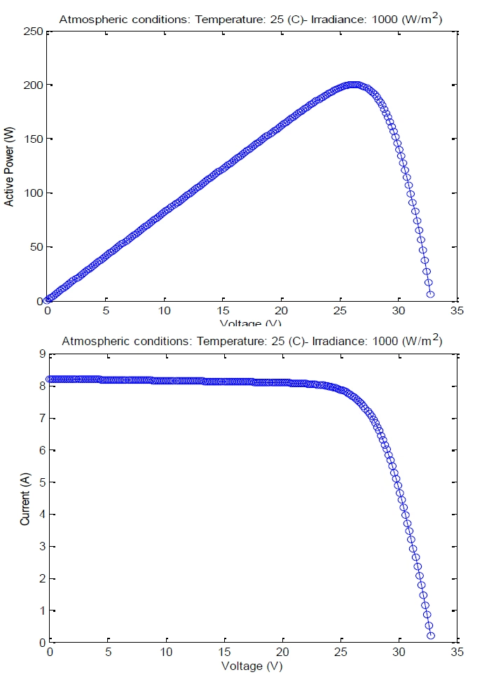
Two curves describe the module. The I–V curve relates the output current to the terminal voltage: at low voltage the current is high and almost flat, but near the open-circuit voltage it collapses sharply — so the panel behaves like an ideal current source only over part of its range, and nonlinearly elsewhere. The P–V curve relates output power to voltage, and its key feature is a single peak: the maximum power point. Force too low a dc voltage and the power is below maximum; force too high a voltage and it falls again; there is one optimal voltage region where the power is greatest — and that peak is the operating point the MPPT control tries to follow.

PV module characteristics at 25 C and 1000 W/m2: the upper plot is active power versus voltage, rising to a single maximum power point near 200 W at about 26 V then falling; the lower plot is current versus voltage, nearly constant at about 8.2 A then collapsing towards zero near the open-circuit voltage of about 33 V. — Figure 1 — The PV module characteristics: the I–V curve (current nearly constant, then collapsing near open circuit) and the P–V curve with its maximum power point. The inverter chooses where on these curves the module operates.

Section 4

Why changing the dc voltage changes the power

This is the central physical idea. Power is the product of voltage and current, but the current is itself a function of the voltage along the I–V curve, so moving the dc operating voltage moves the product:

\[ P = V_{pv}\,I_{pv}, \qquad \left.\frac{dP}{dV_{pv}}\right|_{\mathrm{MPP}} = 0 \]

\(P\): PV output power
\(V_{pv},I_{pv}\): PV terminal voltage and current (with \(I_{pv}\) a function of \(V_{pv}\))
\(\mathrm{MPP}\): maximum power point, where the slope of the P–V curve is zero

Maximum-power-point tracking is exactly this: choose the dc voltage that places the panel at the top of its P–V curve. To take more or less active power, the inverter simply moves the dc operating point — the source obliges according to its characteristic.

Section 5

Irradiance and temperature move the curve

The characteristic is not fixed once and for all; it moves with the weather. The two dominant influences are irradiance and temperature. More irradiance means more photocurrent and usually more available power, lifting the I–V curve upward; the photocurrent scales with irradiance and is corrected for temperature through the short-circuit-current coefficient:

\[ I_{ph} = \big(I_{sc} + K_i\,\Delta T\big)\,\frac{G}{G_{ref}}, \qquad \Delta T = T - T_{ref} \]

\(I_{ph}\): photocurrent at the operating condition
\(I_{sc}\): short-circuit current at standard test conditions
\(K_i\): temperature coefficient of short-circuit current
\(G,\ G_{ref}\): operating and reference irradiance
\(\Delta T\): temperature rise above the reference \(T_{ref}\)

Temperature mainly affects the diode behaviour and the open-circuit voltage (through the coefficient \(K_v\)), reshaping the curve, while irradiance scales the photocurrent. So the panel characteristics shift continuously with conditions — another reason a fixed source will not do.

Section 6

The single-diode equivalent circuit

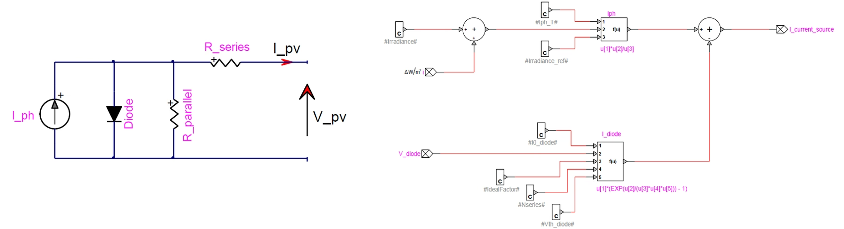
The standard model has four elements: a photocurrent source \(I_{ph}\), a diode, a series resistance \(R_s\) and a parallel (shunt) resistance \(R_p\). Each plays a distinct role in shaping the curve.

Single-diode PV cell model in EMTP: on the left the equivalent circuit, with the light-generated photocurrent source I_ph in parallel with a diode and the shunt resistance R_p (labelled R_parallel), and a series resistance R_s (R_series) to the terminals V_pv and I_pv; on the right the block realisation, where the photocurrent is scaled by irradiance and temperature and the diode current is computed as I0 times exp(V_diode/(a Ns V_T)) minus one, the two combining into the equivalent current source. — Figure 2 — The single-diode PV cell model: a light-generated photocurrent source in parallel with a diode and a shunt resistance \(R_p\), with a series resistance \(R_s\) to the terminals.

Table 1 — The equivalent-circuit elements and what they do.
Element	Represents	Effect on the Curve
\(I_{ph}\)	Light-generated current (the source)	Scales with irradiance; sets the overall current level
Diode	The cell p–n junction	Creates the sharp I–V knee and the nonlinearity
\(R_s\)	Series resistive losses	Voltage drop and fill factor; slope near high current
\(R_p\)	Shunt / leakage path	A higher \(R_p\) reduces leakage current and improves the low-voltage part of the I–V curve

Section 7

The current equation

Applying Kirchhoff’s current law to the equivalent circuit gives the terminal current as the photocurrent minus the diode current minus the shunt-leakage current:

\[ I_{pv} = I_{ph} - I_{diode} - \frac{V_{pv} + I_{pv}R_s}{R_p} \]

\(I_{pv}\): current at the PV terminals
\(I_{ph}\): photocurrent (light-generated)
\(I_{diode}\): current through the diode (the junction)
\(\dfrac{V_{pv} + I_{pv}R_s}{R_p}\): shunt-leakage current through \(R_p\)

Not all of the photocurrent reaches the terminals: some is lost to diode conduction and some leaks through the shunt branch. Because \(I_{pv}\) appears on both sides — inside the diode and leakage terms through the \(I_{pv}R_s\) drop — the equation is implicit in \(I_{pv}\); it cannot be rearranged into a closed form and is normally solved numerically in the model.

Section 8

The diode and the nonlinearity

The diode is what makes the model nonlinear, because its current is exponential in voltage. The Shockley relation for the junction, written for a module of \(N_s\) series cells, is:

\[ I_{diode} = I_0\left[\exp\!\left(\frac{V_{pv} + I_{pv}R_s}{N_s\,a\,V_T}\right) - 1\right], \qquad V_T = \frac{kT}{q} \]

\(I_0\): diode saturation current
\(a\): diode ideality factor
\(N_s\): cells in series per module
\(V_T = kT/q\): thermal voltage (\(k\) Boltzmann, \(q\) electron charge, \(T\) temperature)

This exponential term is why the control-block implementation contains an exponential function, and why a realistic PV source cannot be a linear element. Without the diode the model would miss the sharp I–V knee entirely.

Section 9

Building the model from a datasheet

The practical strength of this approach is that the electrical parameters of the equivalent circuit — which are not given directly in datasheets — can be reconstructed from the quantities manufacturers do publish, with no physical experiments. The standard datasheet set is:

Table 2 — Standard datasheet quantities used to build the model.
Symbol	Quantity	Role
\(P_{max}\)	Maximum power	Anchors the peak of the P–V curve
\(V_{mpp}\)	Voltage at maximum power	Location of the MPP on the voltage axis
\(I_{mpp}\)	Current at maximum power	Current at the MPP
\(V_{oc}\)	Open-circuit voltage	Right-hand end of the I–V curve
\(I_{sc}\)	Short-circuit current	Top-left of the I–V curve; sets \(I_{ph}\)
\(K_i\)	Temp. coefficient of \(I_{sc}\)	Current shift with temperature
\(K_v\)	Temp. coefficient of \(V_{oc}\)	Voltage shift with temperature
\(N_s\)	Cells in series per module	Scales the junction voltage

From these, the software reconstructs the equivalent-cell model — the photocurrent, saturation current and resistances. This is an approximation: the equivalent-circuit parameters are estimated from datasheet values and then used to reproduce the module behaviour around the expected operating range, not to match every measured condition exactly. It is what is needed in practice, since for most studies only datasheet information is available.

The reconstruction is a small root-finding problem. At the maximum-power point the single-diode equation must hold, and the power is stationary there (\(\mathrm{d}P/\mathrm{d}V=0\)); these two conditions let the parallel resistance \(R_p\) and the photocurrent \(I_{ph}\) be written as functions of the series resistance \(R_s\), so the whole fit collapses to a single nonlinear equation \(f(R_s)=0\) that is solved by Newton’s method:

\[ R_s^{\,i+1} = R_s^{\,i} - \frac{f(R_s^{\,i})}{f'(R_s^{\,i})}, \qquad I_0 = \frac{I_{sc}}{\exp\!\big(V_{oc}/(a\,N_s\,V_{T})\big) - 1}, \qquad V_{T}=\frac{kT_{ref}}{q} \]

\(f(R_s)\): residual of the maximum-power-point equation after \(R_p\) and \(I_{ph}\) are substituted as functions of \(R_s\)
\(I_0\): diode reverse-saturation current, fixed by the open- and short-circuit points
\(a,\,V_{T}\): diode ideality factor and thermal voltage (\(k\) Boltzmann constant, \(q\) electron charge, \(T_{ref}\) reference temperature)

Starting the iteration from \(R_s=R_{s,\max}\) converges because \(f\) is monotonic on the bounded interval \([0,\,R_{s,\max}]\); the resulting \(R_s\) then fixes \(R_p\) and \(I_{ph}\). The temperature coefficients \(K_i,K_v\) and the irradiance \(G\) finally scale these standard-test-condition values to the actual operating point, and the per-module figures are multiplied out to the whole array.

Section 10

Standard test conditions

Datasheet figures are quoted at standard test conditions (STC): a reference temperature \(T_{ref}=25\,^{\circ}\mathrm{C}\) and a reference irradiance \(G_{ref}=1000\ \mathrm{W/m^2}\). So the reference I–V and P–V curves are defined at that single operating point, and the model adjusts from there: when the actual temperature and irradiance differ, the temperature corrections, the irradiance scaling and the updated cell behaviour are applied to shift the curves to the real condition. STC is the anchor; the operating-condition corrections do the rest.

Section 11

The module database

Deriving every equivalent-circuit parameter by hand is tedious, so a large PV-module database is a real convenience. If the panel model is already in the database, the software supplies the corresponding module data directly and generates the proper I–V and P–V behaviour, which saves time and improves consistency. In practice you have two routes: enter your own parameters, or select a module from the database — both arrive at the same kind of validated source model.

Section 12

How EMTP® implements it

The PV cell is not represented only by a symbolic diagram; the equation is reproduced with control blocks that actually compute the photocurrent, the diode current, the leakage current and the resulting output current from the nonlinear relation. That is why the implementation contains an irradiance input, the diode-related terms, an exponential function and a final current output — the source is built as a nonlinear current-producing model that drives the dc side. In a converter study that source is then read by the inverter and its converter representation, exactly as the real array would be.

Section 13

The link to the inverter and MPPT

This source model is what gives the inverter its available dc-side power, so the two are tightly coupled. The inverter and its MPPT controller choose a dc operating voltage and current; the PV model says how much current and power are available there; and together they determine the actual active-power injection. You cannot reason correctly about MPPT without the P–V curve behind it — the controller is, quite literally, hunting for the peak of the curve this model produces. The source and the control are two halves of the same problem.

Source and control together

Inverter control picks the dc operating point; the PV model returns the available current and power there. The injected active power is the meeting of the two — which is why MPPT and the P–V curve must be understood as a pair.

Section 14

Key points

A nonlinear source whose operating point sets the power

PV is a nonlinear dc source. A voltage-dependent current source modelled by a single-diode equivalent circuit — photocurrent source, diode, shunt resistance \(R_p\) and series resistance \(R_s\) — not a fixed ideal source.
The I–V and P–V curves define the available power. The terminal current \(I_{pv}=I_{ph}-I_{diode}-(V_{pv}+I_{pv}R_s)/R_p\) gives characteristic curves with a single maximum power point, where \(P=V_{pv}I_{pv}\) is greatest.
Irradiance and temperature shift the curves. The photocurrent scales with irradiance (lifting the I–V curve), while temperature mainly moves the open-circuit voltage — so the curves are not fixed.
The single-diode model explains the curve shape. Its exponential diode current makes the relation nonlinear and implicit; the parameters come from datasheet quantities at STC, or from a module database.
MPPT moves the dc operating voltage. The inverter’s MPPT control chooses the dc voltage that puts the source near the top of its P–V curve, which is how it sets the extracted active power.

The source model and the converter control are two halves of one problem — see the PV park modelling, MPPT control and full-scale converter control guides.

References

EMTP® Documentation and Application Notes. Powersys / EMTP®.

Built on EMTP® · Expert spotlight

Henry Gras

Chief Operating Officer, PGSTech · Montréal, Canada

Henry Gras delivers the EMTP® University course “EMT Simulation and Analysis of Large-Scale Power Systems with Renewables” and works daily with the tool this article is written around.

Henry is based in Montréal, where he is Chief Operating Officer of PGSTech, the company responsible for EMTP® engineering services, commercialisation and continuing software development. He holds a master’s degree from Polytechnique Montréal, where he worked on electrical-machine research, and previously completed an engineering degree at École Centrale de Lyon in France.

Readers who want a structured programme on EMT simulation of large-scale power systems with renewables will find his EMTP® University course an excellent next step.

Henry’s technical expertise covers electromagnetic transient simulation, renewable-energy integration, power-system modelling, electrical machines, protection and specialist transient studies including TRV, transformer energisation, ferroresonance, insulation coordination and power quality.

Part 22 Reading now

PV Cell Single-Diode Source Model

The single-diode equivalent circuit, its I–V and P–V curves, and mapping datasheet parameters onto the model.

Series progress 22 of 30

Part 23

Wind Turbine Aerodynamics and Power Coefficient

The power coefficient Cp, the tip-speed ratio, and the mechanical power source that drives the turbine model.