Renewable Modelling · Turbine Scan, Combined & Verification

The Turbine-Side Impedance Scan and SSCI Verification in EMTP®: Perturbation Extraction, the Combined Scan and Time-Domain Confirmation

The grid-side scan was the easy half. This page does the hard half and closes the loop. The turbine cannot be scanned as an isolated passive element — its impedance depends on the PLL, the operating point and the control mode — so it is connected to an equivalent grid that reproduces the real operating condition, and its impedance is extracted by injecting a current perturbation and measuring the voltage, Z(f)=V(f)/I(f). The turbine resistance comes out negative over much of the range — the dangerous ingredient. Adding the grid and turbine scans, the combined reactance crosses zero near 24–25 Hz with negative resistance, predicting SSCI — and a full time-domain EMT run then confirms a growing oscillation at about 24.5 Hz. This guide walks the turbine scan, the combination, and the verification.

Reading time ≈ 19 min · turbine perturbation scan, combine & verify

The grid-side scan was the easy half: a linear, passive network whose impedance came straight from a fast phasor-domain sweep. This page completes the workflow with the harder half — the converter side — then combines the two signatures and verifies the prediction in full time-domain EMT. With this, the impedance-scan method becomes a complete engineering process: scan, combine, flag, confirm.

Abbreviations used on this page

SSCISub-synchronous control interaction

\(Z(f)\)Frequency-dependent impedance

\(V/I\)Voltage response / injected current

\(R,X\)Resistance, reactance

\(f^{\ast}\)Critical (resonance) frequency

PLLPhase-locked loop

AVMAverage-value model

\(\Delta t\)Measured oscillation period

TDTime domain

EMTElectromagnetic transient

DFIGDoubly-fed induction generator

EMTP®Electromagnetic Transients Program

Key idea

The turbine cannot be scanned as an isolated passive element — its impedance depends on the PLL, the operating point and the control mode — so it is connected to an equivalent grid that reproduces the real operating condition, and its impedance is found by injecting a current perturbation: \(Z(f)=V(f)/I(f)\).
The perturbation is kept near the real operating current (the control is nonlinear), the model is initialised once and scanned from the settled state, and an averaging period is applied. The turbine resistance comes out negative over a wide band — the dangerous ingredient.
Adding the scans gives \(R_{total}=R_{grid}+R_{turbine}\) and \(X_{total}=X_{grid}+X_{turbine}\). The system is flagged where \(X_{total}=0\) (resonance) and \(R_{total}\lt 0\) there (negative damping). In the example, the reactance crosses zero near 24–25 Hz.
A full time-domain EMT run then shows a growing subsynchronous oscillation; its period measured with cursors gives about 24.5 Hz — confirming the scan. Scan to predict, EMT to confirm.

Key terms used on this page

01Turbine-side impedance

The converter, control and filter impedance \(Z_{turbine}(f)\) seen from the interface.

02Equivalent grid

A grid model chosen so the turbine operates at the same point as in the real network.

03Perturbation injection

A small sinusoidal current added at each frequency to measure the voltage response.

04Operating point

The current, power, control mode and PLL state at which the impedance is measured.

05Linearisation

The small-signal impedance is valid only near the operating point it is measured at.

06Initialise once

Settle the model once, save the state, and scan onward without re-settling at every frequency.

07Averaging period

A window used to extract the effective component when harmonics or residual oscillation remain.

08Negative resistance

A turbine \(R_{turbine}\lt 0\): the converter contributes negative damping at those frequencies.

09Combined scan

The sum of grid and turbine impedances, plotted as \(R_{total}(f)\) and \(X_{total}(f)\).

10Zero crossing

The frequency where \(X_{total}=0\); the resonance candidate to test for negative resistance.

11Time-domain verification

A full EMT run that confirms whether the flagged mode actually grows, and at what frequency.

12Cursor measurement

Reading the oscillation period \(\Delta t\) off the waveform to get its frequency \(1/\Delta t\).

Section 1

Completing the workflow

The combined-scan idea needs both halves. The grid half was straightforward; this page builds the turbine half, combines them, and then closes the loop with a full time-domain check. That final verification is what turns the impedance scan from a screening interpretation into a result you can stand behind: the scan predicts the mode, and the EMT case proves it.

Scan to predict, EMT to confirm

The combined impedance scan flags a candidate frequency cheaply; the full time-domain EMT run confirms whether the oscillation actually grows, and at what frequency. The two together are the complete method.

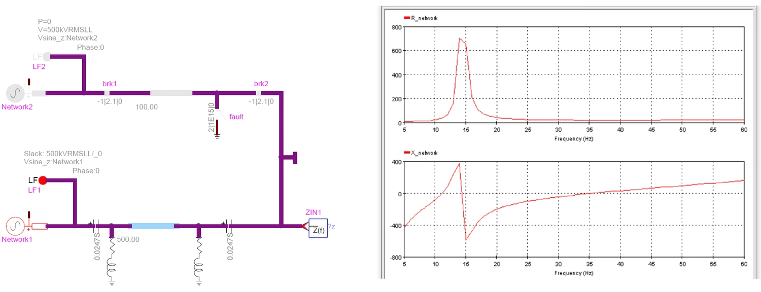
Grid-side impedance scan in EMTP: the linear network seen from the wind-park terminals — slack sources, line breakers, a series-compensated feeder and the fault that reconfigures it — with the Input Impedance frequency-scan probe, and the resulting grid resistance R_network and reactance X_network versus frequency, showing a sharp series-resonance peak near 14 to 15 Hz where the reactance passes through zero. — Figure 1 — The grid-side scan (step 1, recap): the linear network seen from the park terminals and its resistance and reactance versus frequency, with a series-compensation resonance near 14–15 Hz. This is the “easy” half, done in the phasor domain; the turbine half is built below.

Section 2

Why the converter side is harder

For the grid, life was easy: the external network was linear and passive, so a phasor-domain scan gave \(R_{grid}(f)\) and \(X_{grid}(f)\) directly and quickly. The turbine is a different animal — nonlinear, converter-controlled, and dependent on the PLL, the filters, the operating point, the limits and the control mode. You cannot isolate it like a passive RLC network and run a simple phasor scan, and it cannot even operate by itself: it needs a grid reference to synchronise the PLL, establish the operating point and inject the right active and reactive power. That forces a more careful procedure:

Table 1 — What the turbine-side scan requires, and why.
Requirement	Why
Connect an equivalent grid	The turbine cannot run alone; it needs a grid to synchronise the PLL and set the operating point
Match the operating condition	The converter impedance depends on the operating point; the wrong point gives the wrong signature
Perturb near the operating current	The control is nonlinear; perturbing too far measures the wrong linearisation
Initialise once, scan from settled	Avoids re-settling the PLL and dc link at every scan frequency
Apply an averaging period	Harmonics and residual oscillation mean the response is not a single pure tone

Section 3

Connecting an equivalent grid

To scan the turbine properly it is connected to an equivalent grid that reproduces the same conditions it sees in the real network — the same voltage, the same active and reactive power, and effectively the same external impedance environment. So the scan is not done on a “floating” turbine but on one placed in its correct operating context. This matters precisely because the converter impedance depends on the operating point: scan it at the wrong operating point and you get the wrong impedance signature.

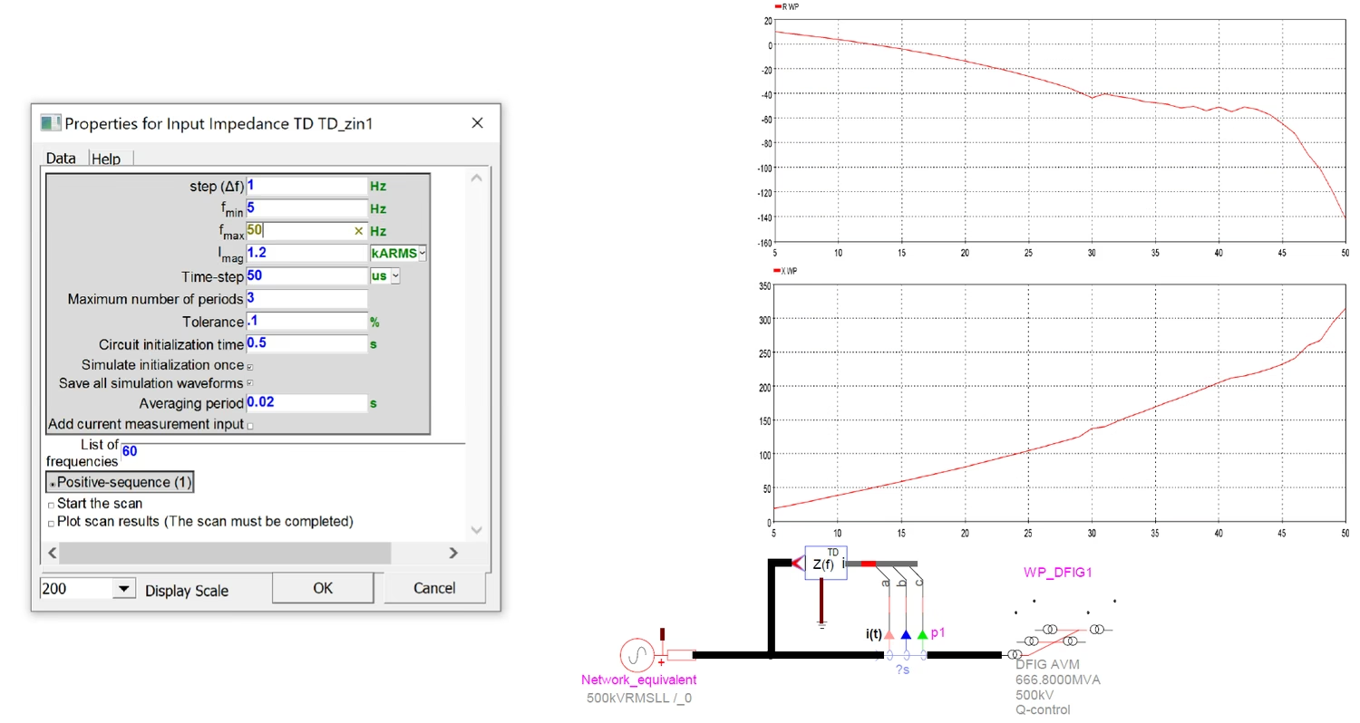
Turbine-side scan in EMTP: the Input Impedance TD device mask (frequency step 1 Hz, 5 to 50 Hz, 1.2 kA RMS perturbation, 50 microsecond time-step, 0.5 s initialisation, positive sequence, 60 Hz filtered out); the equivalent-grid test circuit with the DFIG average-value model connected to a network equivalent and the impedance probe with current injection at the interface; and the resulting turbine resistance R_WP and reactance X_WP versus frequency, the resistance turning negative across much of the 5 to 50 Hz band. — Figure 2 — The turbine-side scan in EMTP®: the Input Impedance TD device settings, the equivalent-grid test circuit with the impedance probe and current-perturbation injection at the DFIG interface, and the resulting turbine resistance and reactance — note the resistance going negative over much of the band.

Section 4

Extracting the impedance by perturbation

With the turbine at its correct operating point, the impedance is measured the direct way: inject a small current perturbation and observe the voltage response. For each scan frequency, the ratio of voltage to current is the impedance at that frequency:

\[ Z_{turbine}(f) = \frac{V(f)}{I(f)} = R_{turbine}(f) + jX_{turbine}(f) \]

\(I(f)\): injected sinusoidal current perturbation at frequency \(f\)
\(V(f)\): measured voltage response at that frequency
\(R_{turbine},X_{turbine}\): turbine-side resistance and reactance

Repeating this across the frequency range builds the turbine signature \(R_{turbine}(f)\) and \(X_{turbine}(f)\) point by point — the same idea as the grid scan, but carried out in time domain because the turbine is an active, controlled element.

Section 5

Perturb around the operating current

There is a subtle but important rule about the perturbation: it must be applied close to the correct operating region, around the real current level. The turbine impedance is not a fixed property like a resistor; it depends on the operating current, the power output, the controller and PLL state, and the reactive control mode. So if you perturb too far from the real operating point, you are measuring the wrong linearisation — effectively scanning the wrong area of the turbine’s behaviour. Keeping the perturbation near the real current is what makes the measured impedance representative of the actual operating condition.

Section 6

Initialise once, then scan

A converter model takes time to settle — the PLL must lock, the controllers and the dc link must reach steady state — which can be half a second, a second, or more. Restarting that from zero at every scan frequency would make the process painfully slow. So the tool initialises once, saves the settled operating point, and then continues scanning from that state, frequency by frequency. The mask exposes exactly these controls:

Table 2 — Representative turbine-side scan settings (illustrative).
Parameter	Value	Role
Frequency step \(\Delta f\)	1 Hz	Scan resolution
\(f_{min}\) – \(f_{max}\)	5 – 50 Hz	Subsynchronous window
Perturbation magnitude	1.2 kA (RMS)	Near the operating current
Time-step	50 µs	EMT integration step
Circuit initialisation time	0.5 s	Settle PLL and dc link (once)
Averaging period	0.02 s	Extract the effective component
Sequence	Positive	The sequence scanned

Section 7

Why averaging is needed

An averaging period is applied because, in a real converter model, the response at the scan frequency may not settle to a perfectly constant sinusoid. The waveform can contain harmonics, some residual oscillation may remain, and the “steady state” is rarely a single pure tone. Averaging over a defined window extracts the effective component at the scan frequency more robustly, which makes the impedance estimate cleaner and more reliable than reading a single noisy cycle would allow.

Section 8

The turbine signature: negative resistance

The turbine-side result has one feature that matters above all: the resistance \(R_{turbine}(f)\) becomes negative over a large part of the scan range. Negative resistance means the converter is contributing energy — acting with negative damping — at those frequencies. That does not by itself prove instability, because the grid side still matters, but it is the dangerous ingredient: a converter with the potential to drive oscillations if a grid resonance happens to align with it. The whole point of combining the two scans is to see whether such an alignment exists.

Section 9

The combined scan

The grid and turbine signatures are now added — resistances together, reactances together — and plotted as the total. Then the combination is screened for the instability signature:

\[ R_{total}(f) = R_{grid}(f) + R_{turbine}(f), \qquad X_{total}(f) = X_{grid}(f) + X_{turbine}(f) \] \[ \text{flag } f^{\ast}: \quad X_{total}(f^{\ast}) = 0 \ \ \text{and} \ \ R_{total}(f^{\ast}) \lt 0 \]

\(R_{total},X_{total}\): combined resistance and reactance versus frequency
\(f^{\ast}\): frequency where the total reactance crosses zero

The combined plot shows \(R_{total}\) and \(X_{total}\) together; the critical step is to find where \(X_{total}\) crosses zero (the resonance) and then check the sign of \(R_{total}\) there.

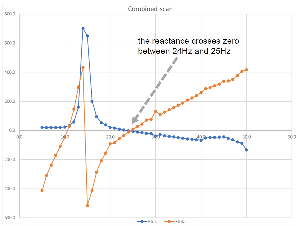
Combined scan in EMTP: total resistance R_total and total reactance X_total versus frequency from 5 to 50 Hz, formed by adding the grid and turbine scans. The reactance crosses zero between 24 and 25 Hz, and at that crossing the total resistance is negative — the predicted sub-synchronous control interaction mode. — Figure 3 — The combined scan: total resistance and total reactance versus frequency. The reactance crosses zero near 24–25 Hz with the resistance negative there — a predicted SSCI mode.

Section 10

Reading the zero crossing

A common confusion is worth clearing up: you are not looking for the \(R\) curve to cross the \(X\) curve, nor for both to be zero at the same point. You are looking for the frequency where \(X_{total}=0\), and then asking whether \(R_{total}\lt 0\) at that same frequency. The zero crossing of the reactance defines the resonance point; the sign of the resistance there tells you whether that resonance has negative damping. So where the two plotted lines happen to intersect each other is irrelevant. In the worked example, the reactance crosses zero between about 24 and 25 Hz, and the resistance there is negative — so the scan predicts potential SSCI near 24.5 Hz.

The prediction

\(X_{total}=0\) near 24–25 Hz with \(R_{total}\lt 0\) there → a predicted SSCI mode around 24.5 Hz, to be confirmed in time domain.

Section 11

Time-domain verification

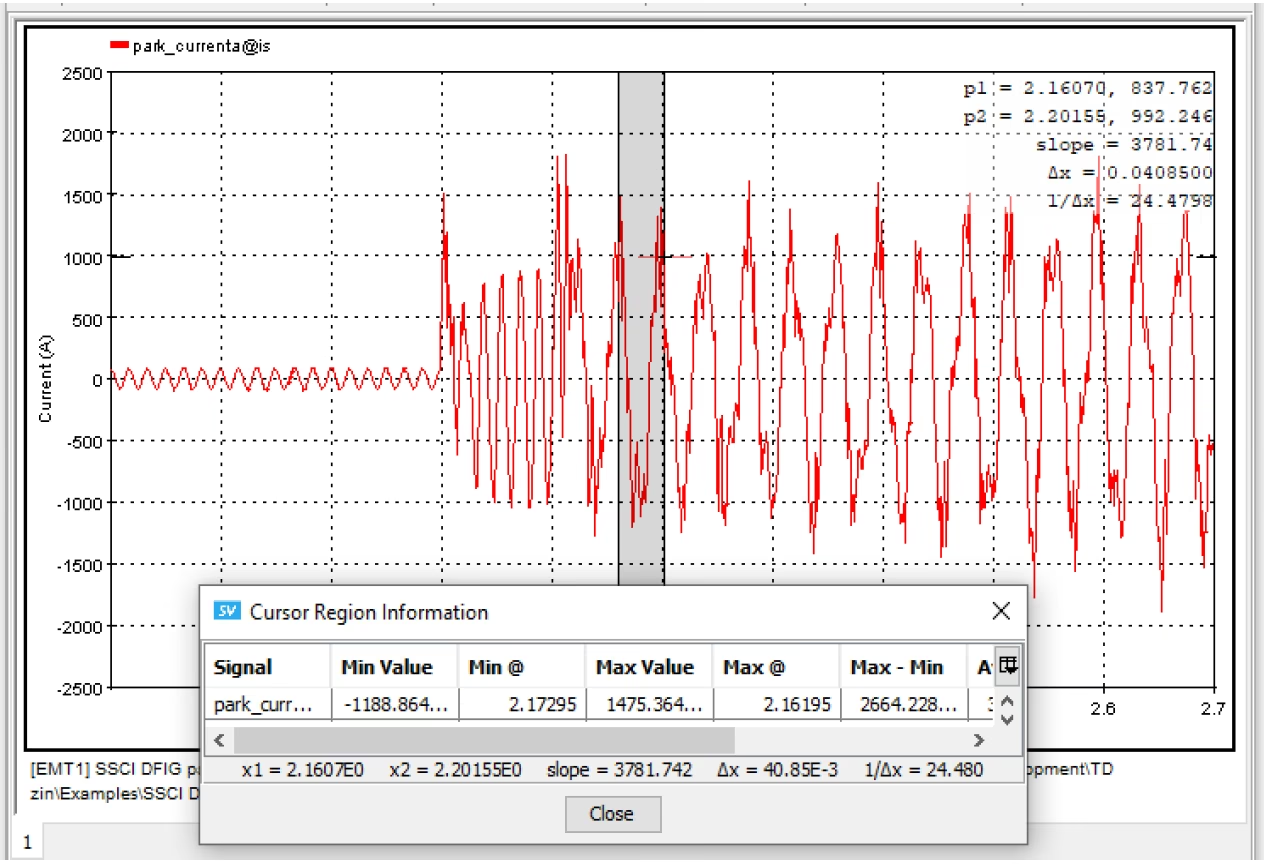
However powerful, the combined scan is a screening, small-signal interpretation; the final proof is a full time-domain EMT run, which tells you whether the oscillation actually grows, what its waveform looks like, how severe it is, and whether the predicted frequency is really present. The verification case here shows the park current starting out normal and then, after the topology change, developing a growing oscillatory component — the signature of SSCI. Reading the period off the waveform with cursors gives the frequency:

\[ f_{osc} = \frac{1}{\Delta t} \approx \frac{1}{0.0409\ \text{s}} \approx 24.5\ \text{Hz} \]

\(\Delta t\): measured period of the growing oscillation (from the cursors)
\(f_{osc}\): oscillation frequency

The measured oscillation, about 24.5 Hz, matches the combined-scan prediction of 24–25 Hz very closely — a strong validation that the scan identified the real mode.

Time-domain EMT verification: the wind-park current versus time, small and steady until about 2.1 s, then growing into a large sub-synchronous oscillation after the line disconnects. The cursor readout gives a period of 0.04085 s, i.e. 24.48 Hz, confirming the combined-scan prediction near 24.5 Hz. — Figure 4 — Full EMT verification: the park current grows into a subsynchronous oscillation whose measured period corresponds to about 24.5 Hz, confirming the combined-scan prediction.

Section 12

What the negative resistance physically means

It is worth stating the mechanism plainly. At the dangerous frequency, the turbine’s converter control is effectively contributing negative damping: the grid provides a resonant electrical structure, and the converter control feeds energy into that mode instead of removing it. So SSCI is not simply “a resonance exists”; it is a resonant network mode plus a converter that energises that mode. That is exactly why both scans are needed — the grid scan finds the resonance, the turbine scan finds the negative damping, and only the combination reveals whether they coincide.

Section 13

Key points

The complete impedance-based SSCI workflow, end to end:

Scan the grid side quickly in the phasor domain (linear, passive).
Scan the turbine side in time domain, on an equivalent grid, around the actual operating point.
Combine the two signatures into \(R_{total}\) and \(X_{total}\).
Flag frequencies where \(X_{total}=0\) and \(R_{total}\lt 0\).
Verify only the flagged cases with targeted EMT time-domain runs.

Predicted and confirmed — The turbine impedance is extracted by perturbing the converter on an equivalent grid at its real operating point, giving \(Z_{turbine}(f)=V(f)/I(f)\) with a resistance that is negative over a wide band. Added to the grid scan, the combined reactance crosses zero near 24–25 Hz with negative resistance — a predicted SSCI mode — and a full time-domain EMT run confirms a growing oscillation at about 24.5 Hz. The method is efficient because the heavy time-domain run is reserved for the few flagged conditions. For the rest of the workflow, see the impedance-scan method, the grid-side scan, the SSCI parameter and the wind-park modelling guides.

References

EMTP® Documentation and Application Notes. Powersys / EMTP®.

Built on EMTP® · Expert spotlight

Henry Gras

Chief Operating Officer, PGSTech · Montréal, Canada

Henry Gras delivers the EMTP® University course “EMT Simulation and Analysis of Large-Scale Power Systems with Renewables” and works daily with the tool this article is written around.

Henry is based in Montréal, where he is Chief Operating Officer of PGSTech, the company responsible for EMTP® engineering services, commercialisation and continuing software development. He holds a master’s degree from Polytechnique Montréal, where he worked on electrical-machine research, and previously completed an engineering degree at École Centrale de Lyon in France.

Readers who want a structured programme on EMT simulation of large-scale power systems with renewables will find his EMTP® University course an excellent next step.

Henry’s technical expertise covers electromagnetic transient simulation, renewable-energy integration, power-system modelling, electrical machines, protection and specialist transient studies including TRV, transformer energisation, ferroresonance, insulation coordination and power quality.

Part 28 Reading now

The Turbine-Side Scan and SSCI Verification

Perturbation extraction, the combined scan and time-domain confirmation of the SSCI result.

Series progress 28 of 30

Part 29

EMT versus RMS for Weak-Grid Converter Instability

Why weak-grid converter instability needs EMT: SCR, the GSC current loop and PLL dynamics.