Renewable Modelling · Full-Scale Converter

Full-Scale Converter Control in EMTP®: Full-Converter Wind and PV with MSC, GSC and dq Control

Move from the DFIG to the full-scale converter and the control gets cleaner, because now all the plant’s power flows through the converter and the dc link largely separates the source from the grid. This is the grid-facing structure shared by full-converter wind turbines and PV plants: a source-side converter, a dc link, a grid-side converter and an interface filter. Because it aligns its control to the grid with a phase-locked loop, it is a grid-following converter. This guide follows the control from measurement through the PLL and the dq transformation — the step that makes active and reactive power approximately separable and lets simple PI control work — to the source-side and grid-side converters, with pitch and protection alongside.

Reading time ≈ 22 min · FSC, MSC/GSC, PLL & dq control

The DFIG converter-control guide looked at a partially-rated converter feeding a machine rotor. The full-scale converter (FSC) is the other major family: here all of the plant’s power passes through an ac–dc–ac converter. This is what full-converter wind turbines and photovoltaic (PV) plants have in common — the grid-facing control structure (measurement, PLL, dq control, inner loops, PWM or average-value action) is essentially shared, even though the source-side physics and controls differ. Because the dc link sits between the source and the grid, the two sides are largely decoupled and the control becomes conceptually cleaner. This guide follows that control from the raw measurements, through the PLL and the dq transformation that make it tractable, to the source-side and grid-side converters — cross-referencing the DFIG page for the detailed dq current loops the two families share.

Abbreviations used on this page

FSCFull-scale converter

FCFull-converter (wind turbine)

PVPhotovoltaic (solar)

MSCMachine-side converter

GSCGrid-side converter

PLLPhase-locked loop

d–q–0Rotating reference frame

PMSGPermanent-magnet synchronous generator

dc linkConverter dc-voltage stage

PWMPulse-width modulation

PIProportional–integral controller

POIPoint of interconnection

FRTFault ride-through

ac / dcAlternating / direct current

puPer unit

\(R+j\omega L\)Converter interface filter impedance

EMTP®Electromagnetic Transients Program

EMTElectromagnetic transient (time domain)

Key idea

A full-scale converter passes all the plant’s power through an ac–dc–ac converter, so the dc link largely decouples the source side from the grid. The control separation is cleaner than in a DFIG, but the response is still bound by the converter controls, current limits and protection. The grid-facing structure is shared by full-converter wind and PV; the source side differs.
The control is layered: measurements & filters → computed variables → source-side (MSC) / grid-side (GSC) control, pitch and protection. The MSC controls machine-side torque and source power extraction (for PV, the dc-side operating point); the GSC holds the dc-link voltage and sets the grid-side active/reactive current.
A PLL gives the grid voltage angle and frequency, so abc quantities become dq0 — this is a grid-following structure. The dq frame makes active and reactive control approximately separable and turns steady-state sinusoids into constants, which simple PI loops drive to zero error.
The converter connects through an interface filter \(R+j\omega L\) around which the current control is designed; the voltage reference is realised by PWM switching or an average-value model. Active/reactive current references are always subject to converter current limits, and during faults the priority may shift toward reactive current. Pitch (wind only) limits power above rated; protection handles cut-in/out, voltage/overcurrent and the dc chopper. The detailed dq loops are as on the DFIG converter page.

Key terms used on this page

01Full-scale converter

A converter that processes the whole plant output, largely decoupling the source from the grid through the dc link.

02Machine-/source-side converter

The MSC: controls the source side — for wind the generator electromagnetic torque, for PV the dc-side operating point.

03Grid-side converter

The GSC: maintains the dc-link voltage and sets the grid-side active/reactive current (voltage/reactive support via that current reference).

04dc-link decoupling

The dc link largely separates source-side and grid-side dynamics, linking them through dc-link power balance.

05Measurements & filters

The signal-conditioning stage: voltages, currents, speed and dc voltage measured and low-pass filtered.

06Compute variables

Derives the controller’s internal variables — dq components, powers, angle and frequency.

07PLL

Phase-locked loop: estimates the grid voltage angle and frequency that define the rotating frame.

08dq transformation

Maps three-phase abc quantities to a rotating frame where balanced steady-state values are constant.

09Decoupled control

Using the dq frame so one channel handles active and the other reactive power, controlled separately.

10Pitch control

Wind-only: increases blade pitch above rated wind to limit the mechanical power captured.

11Protection system

Cut-in/out logic, voltage and overcurrent protections, dc chopper and breaker control.

12Interface filter

The \(R+j\omega L\) reactor between converter and grid through which the current is shaped.

Section 1

One structure for full-converter wind and PV

The full-scale converter is the topology behind both full-converter wind turbines and PV plants. Their energy sources differ — a wind turbine with a generator, or a PV dc source — and the source-side controls differ with them, but the grid-facing control is essentially shared: measure, lock onto the grid with a PLL (making this a grid-following converter), transform to dq, control active and reactive behaviour in dq, let the inner loops produce voltage references, and realise them by PWM switching or an average-value model. That shared grid-facing framework is the subject of this page; the source-specific parts are noted where they differ. For the PV plant context see the PV-park guide.

Different sources, one grid-facing framework

The grid-side behaviour — PLL, dq transformation, approximately decoupled active/reactive control, inner current loops and PWM or average-value action — is common to full-converter wind and PV. The source side is where they differ.

Section 2

The full-scale converter topology

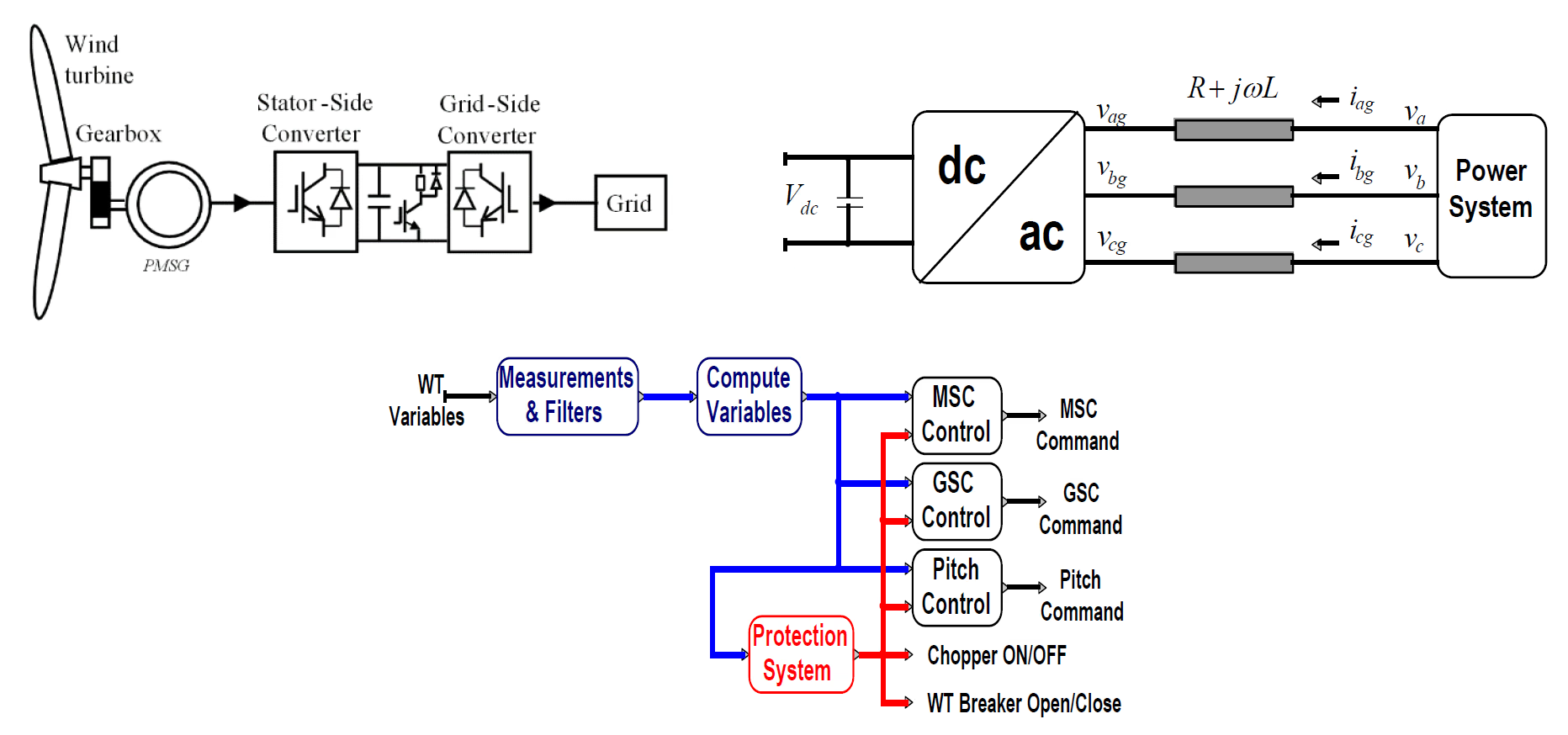
For a full-converter wind turbine the chain is: wind turbine, an optional gearbox (many modern turbines are direct-drive without one), a generator — often a permanent-magnet synchronous generator (PMSG), though other generator types are used behind a full converter — a machine-side converter, a dc link, a grid-side converter, and the grid. For PV there is no rotating machine: the source side is a PV source / dc-side representation, which may feed the inverter directly or through a dc–dc stage depending on the model, then the dc link, the inverter, an interface filter and the grid. The generic grid-facing picture is two voltage-source converters — one facing the source, one facing the grid — separated by a dc link, with the grid side connected through an interface impedance \(R+j\omega L\).

Full-scale converter topology: the source — a generator for full-converter wind, or a PV dc source — feeds a machine-side (source-side) converter; a dc link separates the two sides; and a grid-side converter connects to the power system through the interface filter R + jwL. — Figure 1 — The full-scale converter. The source (a generator for full-converter wind, or a PV dc source) feeds a machine-side (source-side) converter; a dc link separates the two sides; and a grid-side converter connects to the grid through the interface filter \(R+j\omega L\).

Section 3

Why the dc link makes control easier

The full converter is conceptually simpler than a DFIG for one reason: the dc link provides a strong dynamic buffer between the two sides. In a DFIG the stator is connected directly to the grid and the rotor is converter-controlled, so the machine and the grid are partly coupled. In a full-scale converter all the power passes through the converter, so the dc link largely separates source-side and grid-side dynamics — the source does not directly “see” the grid, and the grid sees the source only through the converter. The two sides are not completely independent, though: they stay coupled through the dc-link energy, the power balance, the controller limits and the protection actions.

Instead of one partly-coupled electromechanical-and-grid problem, you get two converter problems linked by dc-link power balance: the machine-side converter can concentrate on the source, and the grid-side converter on grid support and dc-link regulation. The dc-link voltage is the observable result of that balance — if the source-side power exceeds what the grid side exports the dc voltage rises, and if grid export exceeds the source input it falls — which is exactly why the grid-side converter regulates it. The separation makes the control cleaner than in a DFIG, but the response is still limited by the converter controls, the current limits and the protection logic.

Two problems, one dc link

The dc link is the real decoupling element: it turns the plant into a machine-side control problem and a grid-side control problem, joined only by the requirement that dc-link power in equals power out.

Section 4

The control architecture

The control is organised as a clear sequence of signal processing rather than a tangle of blocks. Measured signals are filtered, internal variables are computed from them, and those variables feed the control and protection functions:

Measurements & Filters — condition the raw signals.
Compute Variables — derive the controller’s internal quantities.
MSC Control — machine-side converter commands.
GSC Control — grid-side converter commands.
Pitch Control — blade-pitch command (wind only).
Protection System — chopper, breaker and abnormal-condition logic.

Figure placeholder The full-scale converter control architecture Image to be inserted — the control block diagram: WT variables → Measurements & Filters → Compute Variables, feeding MSC control, GSC control, pitch control and the protection system (chopper / breaker).

Figure 2 — The full-scale converter control architecture: measured turbine variables are filtered and turned into computed variables, which feed the machine-side and grid-side converter controls, the pitch control and the protection system in parallel.

Section 5

Measurements and filters

The first stage measures and conditions the signals the controller needs — phase voltages and currents, machine speed, and the dc-link voltage — and passes them through low-pass measuring filters. Raw instantaneous signals contain switching-frequency components, harmonics and transient content that are not always suitable for direct use in the slower supervisory control loops, so the filters remove that switching ripple, numerical noise and high-frequency content before the variables are used. Filtering is not free: it adds delay, which can matter for weak-grid and fast-transient response, so the filter time constants are a design trade-off between clean signals and speed. The rule downstream is always measure → filter → prepare for control use, and everything after this stage depends on it.

Section 6

Compute variables

The conditioned measurements are then turned into the internal variables the control loops actually use. The controller rarely works with raw abc voltages directly; it works with transformed and derived quantities. Concretely, the main computed variables are the dq voltages \(v_d,\ v_q\) and currents \(i_d,\ i_q\); the active and reactive power \(P\) and \(Q\); the positive-sequence voltage; the PLL angle and frequency; the dc-link voltage error; the current-reference limits; and the protection flags. This “compute variables” block sits between measurement and the control loops precisely to produce those quantities.

Section 7

The PLL: finding the rotating frame

A phase-locked loop (PLL) gives the controller two things: the grid voltage angle and the corresponding synchronous frequency. These are needed because dq control is rotating-frame control — to define the d and q axes meaningfully, the controller must know how the electrical frame is rotating. The PLL supplies that reference angle, and the abc signals can then be transformed into dq quantities aligned with the grid. Because the whole structure is anchored to the PLL angle, this is a grid-following converter; grid-forming control, which builds its own angle, is a different architecture outside this page’s scope. One caution: the PLL is only as clean as the voltage it tracks. During severe voltage dips, harmonics or unbalance, and on weak grids, the estimated angle can become noisy or lag, and PLL behaviour then strongly shapes the weak-grid, unbalanced-fault and low-voltage transient response — so the PLL is often where converter-stability problems begin.

Section 8

abc → dq0, and why it helps

With the angle from the PLL, the phase-domain abc signals are transformed into the rotating dq0 frame — abc quantities mapped onto two rotating axes (\(d\) and \(q\)) plus a \(0\)-axis that carries any zero-sequence content where the model includes it; a controller using only positive-sequence dq works with \(d\) and \(q\) alone. The transformation earns its keep for two reasons. First, it makes active and reactive control approximately separable. Under balanced conditions, correct frame alignment and no limiting interaction, one current component is associated mainly with active power and the other with reactive power, so a single complicated three-phase problem becomes two simple scalar channels. With the frame aligned so the voltage lies on the d-axis (\(v_q=0\)), and using the convention that positive \(P\) and \(Q\) are injection from the plant into the grid:

\[ P = \tfrac{3}{2}\,(v_d i_d + v_q i_q), \qquad Q = \tfrac{3}{2}\,(v_q i_d - v_d i_q) \;\;\xrightarrow{\,v_q=0\,}\;\; P = \tfrac{3}{2}\,v_d i_d,\quad Q = -\tfrac{3}{2}\,v_d i_q \]

\(P,\ Q\): active and reactive power at the converter terminals (positive = injection into the grid, in this convention)
\(v_d,\ v_q\): dq components of the terminal voltage
\(i_d,\ i_q\): dq components of the current
\(v_q=0\): frame aligned to the voltage — then \(P\propto i_d\) and \(Q\propto -i_q\)

Aligning the frame to the voltage makes active power depend on \(i_d\) and reactive power on \(i_q\) — the basis of (approximately) decoupled vector control, one loop for each. Mind the negative sign in \(Q=-\tfrac{3}{2}v_d i_q\): the sign of \(Q\) depends on the reactive-power sign convention and the chosen dq-axis definition, so always check the convention before reading a sign off the diagram.

Second, steady-state quantities become constant. Where the abc voltages and currents are sinusoids that change continuously, in a correctly rotating dq frame the same balanced steady-state quantities become near-constant. A controller regulates constants far more easily than sinusoids: the objective reduces to driving a steady error \(e = x^{*}-x\) to zero, which a simple PI does naturally. Trying to track sinusoidal references directly in the time domain is much harder. So the dq transformation turns an ac tracking problem into a quasi-dc regulation problem — the reason PI-based converter control is so effective.

Section 9

MSC and GSC: splitting the job

The two converters divide the work cleanly, each controlled in dq form for its own objective.

Table 1 — The two converters of a full-scale converter and their control objectives. MSC = machine-side (source-side) converter; GSC = grid-side converter.
Converter	Side	Main objective	Also
MSC (machine-/source-side)	Source / machine	Generator torque and source power extraction — it does not directly control grid reactive power	For PV: the source-side dc operating point (no torque loop)
GSC (grid-side)	Grid	dc-link voltage, plus grid-side active and reactive current to plant-level requirements	Voltage / reactive support delivered through the grid-side current reference, within capability limits

The MSC row applies mainly to full-converter wind (often PMSG-type) models; a PV plant may instead have a dc-side source and controller rather than a machine-side converter. Any “terminal voltage” support the GSC provides is achieved through its current reference and is bounded by converter capability — and note that plant-level reactive/voltage targets are usually measured at the POI by the plant controller, while the local GSC works from converter- or turbine-terminal measurements.

So one converter controls the source / machine side and the other the grid interface. The detailed structure of each — an outer loop producing a dq current reference, a current limiter, and a fast inner current loop producing the voltage reference realised by PWM or an average-value model — is exactly the cascade developed on the DFIG converter-control page; only the objectives assigned to the dq axes differ between the families.

Section 10

Pitch control and the protection system

Two further blocks complete the architecture. Pitch control applies to the wind case only: above rated wind speed it increases the blade pitch angle to limit the mechanical power captured and keep the turbine within safe limits. It is a slow mechanical power-limiting loop, separate from and much slower than the fast electrical current-control loops. A PV plant has no blades and no generator torque loop; its source-side control is dc-power / MPPT / curtailment related, and its available active power is set by irradiance, temperature, MPPT, curtailment, the inverter rating and dc-link limits rather than by pitch.

The protection system handles abnormal conditions rather than normal operation. Depending on the model it may include cut-in and cut-off logic, over- and under-voltage protection, overcurrent protection, current limiting, converter blocking, breaker control, ride-through logic and a dc chopper — not every project model contains all of these, or implements them the same way. The dc chopper is worth singling out: it dissipates excess dc-link energy when the grid-side converter cannot export enough power during a fault or transient, protecting the dc link from over-voltage. Protection is fed from the same measurement and filtering stage as the control loops, which is why it sits within the common signal-processing framework rather than off to one side.

Section 11

The interface filter \(R+j\omega L\)

The grid-side converter does not connect ideally to the grid node; its current is shaped through an interface filter / reactor with resistance \(R\) and inductance \(L\). The current-control equations are built around that filter, because the current produced by a given converter voltage depends on it. In the time-domain dq equations the impedance \(R+j\omega L\) becomes a resistance \(R\), an inductance \(L\) (the \(L\,di/dt\) term), and cross-coupling terms proportional to \(\omega L\) that link the two axes:

\[ v_{cd} = R\,i_d + L\frac{di_d}{dt} - \omega L\,i_q + v_{gd}, \qquad v_{cq} = R\,i_q + L\frac{di_q}{dt} + \omega L\,i_d + v_{gq} \]

\(v_{cd},\ v_{cq}\): converter terminal voltage (dq), the inner loop’s output
\(v_{gd},\ v_{gq}\): grid voltage (dq) at the filter’s far side
\(i_d,\ i_q\): filter / line currents (dq)
\(R,\ L\): interface-filter resistance and inductance
\(L\,di/dt\): inductor voltage from the rate of change of current
\(\omega L\): cross-coupling between the d and q axes (\(\omega\) is the PLL frequency)

The inner current loop computes \(v_{cd},\ v_{cq}\) to make the currents follow their references; the \(\omega L\) cross-terms are usually cancelled by a decoupling feed-forward — which can also include grid-voltage compensation — so the two axes can be tuned nearly independently. The signs of the \(\mp\omega L\) terms follow the chosen Park transformation and current-direction convention, so this is the form used in this model, not a universal one. And “independent” is only approximate: the feed-forward is only as good as the filter parameters, PLL angle and measurements, and the axes stay coupled through limits, saturation, PLL dynamics, weak-grid impedance, digital delay and protection.

Two practical cautions round this out. First, the active and reactive current references are always subject to the converter current limit: the vector of dq current references is capped to the converter’s maximum, and during faults the priority between active and reactive current may shift toward reactive current for voltage support, depending on the grid code and model settings. Second, on weak grids the PLL, current-control and voltage-control interactions become more important, and the standard dq architecture may need careful tuning or added damping to stay stable. Specialised damping or resonance-control functions may be added on top of the core — the PLL, the dq transformation, approximately decoupled active/reactive control and the inner/outer loops — where a particular study requires them.

The shunt harmonic filter alongside the series reactor

The series reactor is only part of the grid-side hardware. Because PWM switching leaves current ripple at and around the switching frequency, a full-converter EMT model typically also places a shunt ac harmonic filter at the grid-side terminal. A representative implementation uses two band-pass branches tuned to the switching-frequency harmonics — the first at the grid-side PWM harmonic order \(n_1 = f_{\mathrm{PWM,gsc}}/f_s\) and the second at its second harmonic \(n_2 = 2\,n_1\) — each with a high quality factor \(Q = 1000\) so the branches are sharply selective at their tuned orders and leave the fundamental essentially untouched. The reactor limits \(di/dt\) and shapes the controlled current; the shunt filter draws off the residual switching-frequency content so the current injected at the point of connection stays clean.

Section 12

Reading the FSC control end to end

Traced as a sequence, the control reads cleanly:

Measure the voltages, currents, speed and dc voltage.
Filter them into reliable control inputs.
PLL — find the grid voltage angle and frequency.
abc → dq0 — transform the phase variables into the rotating frame.
Decouple — control active and reactive behaviour on separate dq channels.
MSC and GSC act on their respective sides (source / machine and grid / dc-link).
Pitch and protection operate alongside — pitch for wind above rated, protection for abnormal conditions.

The dq transformation is the keystone: it is what makes the later detailed PI loops manageable, by decoupling active and reactive control and turning steady-state sinusoids into the constants a PI can regulate to zero.

Section 13

Key points

All the plant’s power passes through the converter, so the dc link largely buffers the source side from the grid — cleaner control than a DFIG, but not fully independent.
The two sides are linked by dc-link power balance: the dc voltage rises or falls with any source-versus-grid power mismatch, which is what the GSC regulates.
A grid-following PLL and the dq transformation make active and reactive control approximately separable and turn steady-state sinusoids into constants a PI can regulate.
The MSC / source-side control handles generator torque or the PV dc operating point; the GSC / grid-side control holds the dc-link voltage and sets grid active/reactive current.
The final response is bounded by current limits and protection, and the voltage reference is realised by PWM switching or an average-value model. The detailed dq loops are as on the DFIG converter page; for the wider plant see the wind-park and PV-park guides.

References

EMTP® Documentation and Application Notes. Powersys / EMTP®.

Built on EMTP® · Expert spotlight

Henry Gras

Chief Operating Officer, PGSTech · Montréal, Canada

Henry Gras delivers the EMTP® University course “EMT Simulation and Analysis of Large-Scale Power Systems with Renewables” and works daily with the tool this article is written around.

Henry is based in Montréal, where he is Chief Operating Officer of PGSTech, the company responsible for EMTP® engineering services, commercialisation and continuing software development. He holds a master’s degree from Polytechnique Montréal, where he worked on electrical-machine research, and previously completed an engineering degree at École Centrale de Lyon in France.

Readers who want a structured programme on EMT simulation of large-scale power systems with renewables will find his EMTP® University course an excellent next step.

Henry’s technical expertise covers electromagnetic transient simulation, renewable-energy integration, power-system modelling, electrical machines, protection and specialist transient studies including TRV, transformer energisation, ferroresonance, insulation coordination and power quality.

Part 8 Reading now

Full-Scale Converter Control

Full-converter wind and PV: the machine-side and grid-side converters and how dq control is split between them.

Series progress 8 of 30

Part 9

Type-4 Wind Turbine MSC Control

MPPT torque, q-axis current and internal-model-control tuning for the machine-side converter.