Renewable Modelling · Plant Controller · Implementation

Plant-Controller Implementation in EMTP®: The Mask, FRT Anti-Windup and Initialisation

The previous guide built the plant controller as a block diagram — the Q, V and PF modes feeding one plant-level reactive-power loop. This one opens the mask. In EMTP® the wind or PV plant controller (PPC; called the wind-park controller, WPC, on a wind park) is a configurable block: you set its gains, limits, output timing, fault ride-through (FRT) thresholds and a Q(V) characteristic. This page is about the practical meaning of those mask fields — not a fresh derivation of plant-level reactive control — and about the three behaviours behind them: a sampled output, anti-windup during faults, and initialisation from the load flow.

Reading time ≈ 18 min · PPC mask, FRT anti-windup & init

In EMTP® the plant controller is reached through a mask — a dialogue of gains, limits, timing and characteristics, and the place where a study is actually parameterised. This guide explains what each field means, then looks more closely at the three that carry real behaviour rather than just a tuning number. It assumes the control logic from the plant-controller reactive power control guide and stays on the implementation.

Abbreviations used on this page
PPCPower-plant (park) controller
WPCWind-park controller
FRTFault ride-through
PIProportional–integral controller
POIPoint of interconnection
PQVCombined active/reactive-power and voltage measurement at the POI
Q(V)Reactive-power vs voltage (Volt-VAR) characteristic
puPer unit
\(K_{Vpoi}\)Outer voltage-control gain
\(K_p,\ K_i\)Proportional and integral gains
\(\Delta U'\)Plant-level voltage-reference correction sent to the local units
ZOHZero-order (sample-and-) hold
EMTP®Electromagnetic Transients Program
EMTElectromagnetic transient (time domain)
Key idea
  1. The PPC is a configurable block exposed through a mask: the gains, limits, output timing, FRT thresholds and the Q(V) curve are all user-set fields, each mapping onto the block-diagram structure. Table 1 lists them.
  2. The output reference is updated in discrete samples (the “voltage reference revise time”), a sample-and-hold reflecting a realistic supervisory timescale; set it to zero for continuous updates.
  3. The FRT logic on the mask is anti-windup. During a deep voltage dip the normal reactive target may be physically unreachable, so the reactive error is held at zero and the integrator frozen — stopping windup and the reactive overshoot that would otherwise follow when the fault clears; pickup and reset thresholds give hysteresis. The full fault response (reactive-current injection, current limiting, priority logic) lives in the local converter control.
  4. The PPC’s own PI is initialised from the load flow, so its integral state already gives the correct output at \(t=0\); without it, even a well-initialised plant starts from a wrong controller output that ramps unwanted into the run. A Q(V) curve adds grid-code Volt-VAR behaviour, and the architecture is open and modifiable.
Key terms used on this page
01PPC mask
The software dialogue exposing the plant controller’s gains, limits, timing and characteristics to the user.
02V-control gain
\(K_{Vpoi}\): how strongly a POI voltage error is turned into a reactive-power request.
03Q-control PI
The plant-level reactive-power regulator; \(K_p\) gives the immediate response, \(K_i\) removes steady-state error.
04Output limits
Maximum / minimum voltage reference, bounding the command sent to the local converters.
05Revise time
The interval at which the output is refreshed and then held (sample-and-hold); zero means continuous.
06Integrator windup
Excessive build-up of a PI’s integral term when it integrates an error the plant cannot satisfy.
07FRT anti-windup
Forcing the error to zero (freezing the PI) during a deep voltage dip so the integrator cannot wind up.
08Pickup / reset
The voltage thresholds to enter and leave FRT handling; different values give hysteresis.
09Q(V) characteristic
A reactive-versus-voltage curve (Volt-VAR): inject at low voltage, deadband near nominal, absorb at high voltage.
10PPC initialisation
Setting the PI integral state (and any sample-and-hold state) from the load-flow solution so the output is correct at \(t=0\).
11Hysteresis
Separate entry and exit thresholds that stop a logic state from chattering around one boundary.
12Open architecture
The controller’s internal logic can be inspected and modified, not just parameterised.

Section 1

From block diagram to a configurable mask

Double-click the plant in the software and a plant-controller tab appears; the mask behind it is the implemented form of the controller described conceptually before. The structure is unchanged — an outer voltage or power-factor function can produce a reactive-power reference, and the plant-level reactive-power PI acts on the POI error and emits a reference correction toward the local converter controls — but now every gain, limit and threshold is a field you can set. This page explains the practical meaning of those fields; the controller is not a black box, but configurable, inspectable and, if a project needs it, modifiable.

Five practical additions

Over the conceptual block diagram, the implementation adds: editable gains and limits; an output updated in discrete samples; FRT logic that prevents bad integrator build-up during faults; a Q(V) characteristic; and initialisation of the controller’s own state from the load flow.

Section 2

The PPC mask: what you can set

The mask gathers the controller’s tunable parameters in one place. The example values below are typical entries; the point is that each maps directly onto the block-diagram structure already described.

Table 1 — The plant-controller mask: the user-set parameters, with example values, their units or base, and what each one sets.
ParameterExampleUnits / baseWhat it sets
V-control gain \(K_{Vpoi}\)1.75pu reactive power per pu voltage errorOuter voltage-loop sensitivity — how strongly a POI voltage error becomes a reactive request.
Q-control gain \(K_p\)1dimensionless (pu \(\Delta U'\) per pu reactive error)Proportional gain of the plant-level reactive-power PI — the immediate response to the POI reactive error.
Q-control gain \(K_i\)2per second (pu per pu·s)Integral gain of the PI — drives the steady-state reactive error to zero.
Max / min voltage reference+1 / −1pu, on the \(\Delta U'\) voltage-reference correctionOutput limits on the voltage-reference correction sent to the local units.
Voltage-reference revise time0.001seconds (0 = continuous)Interval at which the output is refreshed and held (sample-and-hold).
FRT pickup voltage0.175pu voltage deviation from nominalThreshold to enter fault ride-through handling.
FRT reset voltage0.125pu voltage deviation from nominalThreshold to leave FRT handling (gives hysteresis).
Q(V) control curvetablePOI voltage (pu) → reactive command (pu)A reactive-versus-voltage characteristic for grid-code Volt-VAR behaviour.
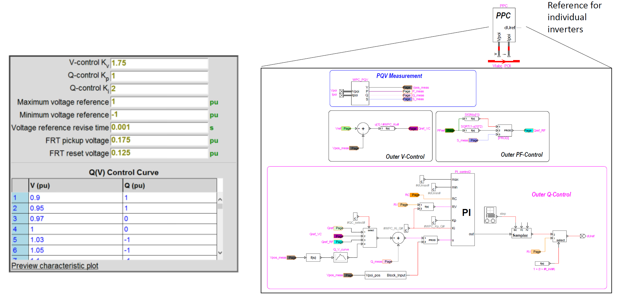
The EMTP plant-controller mask dialogue, showing the V-control gain, the Q-control PI proportional and integral gains, the maximum and minimum voltage-reference limits, the voltage-reference revise time, the FRT pickup and reset voltages, and the Q(V) control-curve fields.
Figure 1 — The plant-controller mask: one dialogue exposing every tunable field of the controller — the gains, limits, output timing, FRT thresholds and the Q(V) curve. Each field maps onto a block of the implemented controller.

Section 3

The V-control gain

The V-control gain \(K_{Vpoi}\) is the gain of the outer voltage loop. It converts the POI voltage deviation \(V'_{POI}-V_{POI}\) — both in per unit, the prime marking the reference and the unprimed symbol the measurement — into a reactive-power reference for the plant-level Q-control PI, not a direct voltage command to the network. With the generator sign convention (positive \(Q\) is injection from the plant into the grid): if the POI voltage is below target the controller raises the reactive-injection request; if it is above target it reduces injection or moves toward absorption. The gain sets how strongly the plant reacts to a voltage error — too low and the correction is sluggish, too high and the plant-level interaction can become aggressive or oscillatory. It is the tuning knob for the plant’s sensitivity in V-control mode.

Section 4

The Q-control PI gains

The plant-level reactive-power PI acts on the error \(Q'_{POI}-Q_{POI}\) and emits the correction sent toward the local units. Its two gains do distinct jobs. The proportional gain \(K_p\) gives an immediate response — a faster, stronger correction for a given error — but too much of it brings overshoot and oscillation. The integral gain \(K_i\) accumulates the error over time and drives the steady-state error to zero, which matters because internal elements (collector grid, cable charging, transformer reactance, shunts) sit between the converters and the POI; the integral action keeps adjusting the output until the measured POI reactive power matches the target. Without it, a steady-state error would remain.

Section 5

Output limits: maximum and minimum reference

The maximum and minimum voltage reference bound the PPC output itself — specifically the plant-level voltage-reference correction \(\Delta U'\) handed to the local units, not the reactive power they ultimately produce. They matter because even if the outer loop or PI “wants” a very large correction during a severe disturbance, the command handed down must stay within a meaningful range; the local controllers are designed to work within a defined reference envelope, so these limits keep the plant-level output sensible. What they do not do is guarantee the response: the final reactive output is still constrained by the inverter/converter current limits, voltage limits, the active-power operating point and the local controller’s own priority logic. The PPC output limit keeps the request reasonable; it does not extend the plant’s physical capability.

Section 6

Sampled output: the “revise time”

One field is easy to overlook but conceptually important: the reference sent to the local units is not revised continuously, it is issued in samples. The voltage-reference revise time is the interval at which the PPC output is recomputed and then held until the next sample — a sample-and-hold (zero-order hold) on the plant-controller output. It is not the simulation time step, and not the converter switching period; it is the supervisory update rate. With a revise time of 0.001 s, for example, the reference is updated every millisecond and held flat in between.

This reflects a real effect: supervisory plant commands are issued at a finite update rate, not continuously and not at the ultra-fast rate of the converter’s inner current loop. A larger revise time makes the PPC act in a visibly stepwise way; a very small one approaches continuous behaviour. Setting the revise time to zero means the output is updated continuously in this EMTP® model — useful for idealised studies, but it removes the realistic supervisory sampling effect. One caution: the revise time alone does not represent the whole communication chain — a real plant also has measurement filtering, communication delay, sampling delay, controller scan time and unit-level response delay, and the revise time captures only the periodic-update part of that picture.

Why it is there

The sampled output captures the practical supervisory timescale — slower than the inner loops — and avoids modelling an unrealistically smooth, infinitely fast plant-level command.

Section 7

FRT mode: anti-windup during voltage dips

The most prominent behaviour on the mask is the fault ride-through (FRT) logic, and on the PPC it is best understood as anti-windup. During a fault the voltage drops sharply and the plant’s normal reactive target may become physically inappropriate or unreachable — the converter current limit, the depressed voltage and grid-code FRT priority now dominate the response — so the measured reactive power diverges from the reference and the PI error becomes large. If the integrator kept integrating that error, its integral term would build up enormously, and when the fault cleared the still-charged integrator would command far too much reactive power, overshooting badly.

\[ \text{during FRT:}\quad e_Q = 0 \;\Rightarrow\; \dot{x}_I = K_i\,e_Q = 0 \]
\(e_Q\)
reactive-power error at the POI — forced to zero while FRT is active
\(x_I\)
integral state of the Q-control PI
\(\dot{x}_I\)
rate of change of the integral state (zero ⇒ frozen)
\(K_i\)
integral gain

In this generic model the anti-windup is implemented by forcing the reactive-error input to zero while FRT is active. With \(e_Q=0\) the integrator rate \(\dot{x}_I=K_i e_Q\) is zero, so the integral state holds at its last value, and the proportional term (also fed by \(e_Q\)) contributes nothing — the output holds rather than winding up. The precise mechanism can differ between implementations (some hold the integrator directly, some clamp the output), but the effect is the same: no wind-up against a target the plant cannot presently meet.

When normal voltage returns the plant resumes from a sensible controller value rather than from an excessively accumulated integral command. It matters most in voltage-control mode, where a deep dip produces a large voltage error that would otherwise become an extreme, unachievable reactive request. One distinction to keep clear, though: this anti-windup is only the PPC’s part of fault ride-through. The actual FRT response of the plant — reactive-current injection, active-current reduction, current limiting, priority logic and protection functions — lives in the local converter control, covered in the grid-side converter FRT guide. The mask setting here only stops the supervisor from winding up.

Section 8

FRT pickup and reset thresholds

FRT handling is entered and left on two voltage thresholds, both expressed as a voltage deviation from nominal. A pickup of 0.175 pu therefore means the measured voltage has fallen 0.175 pu below nominal — down to about 0.825 pu retained voltage on a 1.0 pu base — at which point the PPC enters FRT handling; when the voltage recovers past the reset deviation (for example 0.125 pu, about 0.875 pu retained) it leaves FRT handling and resumes normal error processing. Using two different thresholds gives hysteresis: the controller enters FRT only when the dip is clearly severe and leaves only after a clear recovery, so it does not chatter in and out of the mode when the voltage hovers around a single boundary. Which voltage the thresholds act on matters for unbalanced faults: the generic model compares against a defined measured POI signal — typically the positive-sequence (or RMS) POI voltage rather than an individual phase voltage — so the trigger reflects the balanced severity of the dip, not the worst single phase. Confirm the exact signal for your model version.

Section 9

The Q(V) characteristic

Beyond a single outer-loop gain, the mask lets you define a Q(V) characteristic — a piecewise relationship between POI voltage and commanded reactive power. It is an alternative to the fixed linear V-control gain: both sit on the same voltage-control path and turn a POI voltage into a reactive request, but the Q(V) table replaces the single-gain response with a shaped, non-linear one — a deadband near nominal, saturating injection or absorption at the extremes. You configure one or the other for the voltage response, not both at once. A typical shape injects reactive power at low voltage, does little or nothing in a deadband around nominal, and absorbs reactive power at high voltage:

Table 2 — An example Q(V) (Volt-VAR) characteristic: commanded reactive power (pu, positive = injection into the grid) against POI voltage (pu). The controller interpolates linearly between the listed points.
\(V\) (pu)\(Q\) (pu)Region
0.90+1Low voltage — full reactive injection
0.95+1Low voltage — full reactive injection
0.970Edge of the deadband
1.000Nominal — deadband, no reactive action
1.03−1High voltage — full reactive absorption
1.05−1High voltage — full reactive absorption

A fixed linear gain is simple, but real plants and grid codes often want this kind of non-linear Volt-VAR response. The important caveat is that this curve is a modelled Volt-VAR characteristic: its shape and breakpoints must be set to match the project’s grid-code requirement or the OEM controller settings — the example above is illustrative, not a universally correct curve. And, as everywhere on this page, requesting reactive power does not guarantee delivering it: even if the curve calls for full injection or absorption, the local converter/inverter may not reach it because of current limits, voltage limits, active-power loading or FRT priority.

Section 10

Initialising the PPC

The plant controller contains dynamics of its own — above all the PI integrator — so it too must be initialised, and this is a step separate from initialising the plant. The detailed plant (machines, converters, network) can be initialised perfectly and still be spoiled by the supervisor: start the PPC’s PI with its integral state at zero and its output is wrong at \(t=0\), so it ramps from that wrong value toward the right one and injects an artificial start-up transient into the converter references. The remedy is the same as for every other dynamic state: the PPC is initialised from the load-flow solution. What is set is the PI integral state — and any internal output memory or sample-and-hold state — to the values that make the controller output at \(t=0\) equal the solved steady-state correction, rather than ramping up from zero.

So when the time-domain run begins, the PPC output is already correct, the PI does not have to discover the operating point, and the controller starts from equilibrium. This is consistent with the broader principle covered in the synchronous-machine initialisation guide: not only the network but every dynamic internal state — including the supervisory controller’s — must begin from the correct steady operating condition. It is worth verifying in practice: run the model with no disturbance and confirm that the POI voltage, \(P\), \(Q\), the PPC output \(\Delta U'\), the local-unit references and the measured voltage all stay flat through and after the initialisation window. Any drift there points to an inconsistent controller state.

Why it matters

Controller initialisation is separate from plant initialisation. Even a perfectly initialised plant can be spoiled by an un-initialised supervisor — a wrong initial PI output ripples down to the converters as an unwanted reference ramp. Initialising the PPC closes that last gap.

Section 11

The software architecture

The enlarged software diagram organises these pieces into one signal path: a PQV measurement at the POI (active power, reactive power and voltage) → a mode selector that chooses the active front-end → the V-, PF- and Q-reference formation that turns the operator target into a reactive-power reference \(Q'_{POI}\) → the plant-level Q-control PI acting on the POI reactive error → the FRT anti-windup gate that freezes that PI during a deep dip → the sample-and-hold that applies the revise-time interval → the final reference correction \(\Delta U'\) sent to the local units. It is exactly the architecture described conceptually, now in its implemented, inspectable form.

Figure 2 — The implemented PPC signal flow: a POI PQV measurement feeds the V-, PF- and Q-control functions; a selector picks the active mode, the plant-level Q-control PI acts on the reactive error with FRT anti-windup gating, and a sample-and-hold delivers the reference correction \(\Delta U'\) to the local units. The architecture is open and can be adapted per project.

Section 12

Key points

The mask is not just tuning constants

  1. Mask parameters. The V-control gain, the plant-level Q-control PI gains, the output limits, the revise time, the FRT thresholds and the Q(V) curve are all user-set fields.

  2. Sampled output. The correction is issued as a sample-and-hold at the “revise time”; zero means continuous, but then drops the supervisory sampling effect.

  3. FRT anti-windup. During a deep dip the reactive error is held at zero so the PI cannot wind up; pickup/reset thresholds give hysteresis. The rest of the fault response lives in the converter control.

  4. Q(V) curve. A modelled Volt-VAR characteristic, to be matched to the project grid code — and still bounded by converter capability.

  5. PPC initialisation. The PI integral (and hold) state is set from the load flow, so the output is correct at \(t=0\) and adds no start-up transient.

The PPC mask is not just a list of tuning constants. It defines the plant-level voltage/reactive response, the output sampling, the FRT anti-windup, the Q(V) behaviour and the initial controller state. For reliable EMT studies the PPC must be tuned, limited and initialised consistently with the load-flow operating point and the local converter capability. For the underlying control logic, see the plant-controller reactive power control guide.

References

References

  1. EMTP® Documentation and Application Notes. Powersys / EMTP®.
Built on EMTP® · Expert spotlight
Portrait of Henry Gras, Chief Operating Officer of PGSTech

Henry Gras

Chief Operating Officer, PGSTech · Montréal, Canada

Henry Gras delivers the EMTP® University course “EMT Simulation and Analysis of Large-Scale Power Systems with Renewables” and works daily with the tool this article is written around.

Henry is based in Montréal, where he is Chief Operating Officer of PGSTech, the company responsible for EMTP® engineering services, commercialisation and continuing software development. He holds a master’s degree from Polytechnique Montréal, where he worked on electrical-machine research, and previously completed an engineering degree at École Centrale de Lyon in France.

Readers who want a structured programme on EMT simulation of large-scale power systems with renewables will find his EMTP® University course an excellent next step.

Henry’s technical expertise covers electromagnetic transient simulation, renewable-energy integration, power-system modelling, electrical machines, protection and specialist transient studies including TRV, transformer energisation, ferroresonance, insulation coordination and power quality.

Thirty-Part Technical Series

EMTP® Renewable Energy Modelling

A thirty-part guide to modelling wind, PV and full-converter plant in EMTP® — sources and turbines, converter and plant control, sequence control under faults, protection, and weak-grid and SSCI stability.

Part 6 Reading now

Plant-Controller Implementation and FRT

The plant-controller mask, fault ride-through anti-windup and initialisation of the outer control.

Series progress 6 of 30