Renewable Modelling · Wind Turbine Aerodynamics

Wind Turbine Aerodynamics in EMTP®

Power coefficient, tip-speed ratio and the mechanical power source

The aerodynamic block defines the mechanical power available to a wind-turbine generator before the converter, its control loops or the grid response are considered. In EMTP® this power is calculated from the wind speed, the rotor swept area, the air density, the blade pitch and the power coefficient Cp — so the turbine is a variable-efficiency source, not a fixed one. Because Cp peaks at a single tip-speed ratio, there is one best rotor speed for each wind condition, which is the aerodynamic basis of wind MPPT. What follows builds the aerodynamic source model, sets out the Cp curves and the two control levers — rotor speed and pitch — and shows how the block produces the active-power reference the converter then follows.

Reading time ≈ 18 min · Cp curves, tip-speed ratio & MPPT

Before any electrical power exists, a wind turbine makes mechanical power out of the wind — and it does not do so at a fixed efficiency. The aerodynamic model is the wind counterpart of the PV cell source model: it turns wind speed, rotor speed and blade pitch into shaft power, and every active-power reference the converter later follows is rooted in the power this block produces. Get the aerodynamics right and the rest of the wind study — the converter tracking its power reference — finally has a foundation.

Abbreviations used on this page

WTWind turbine

\(C_p\)Power coefficient (aerodynamic efficiency)

\(\lambda\)Tip-speed ratio

\(\beta\)Blade pitch angle

\(\omega_t\)Turbine rotational speed (rad/s)

\(C_{p,\max}\)Maximum power coefficient

\(\lambda_{opt}\)Optimal tip-speed ratio

\(\rho\)Air density (≈ 1.225 kg/m³)

\(A\)Rotor swept area

MPPTMaximum-power-point tracking

\(K_{opt}\)Optimal-tracking gain

EMTP®Electromagnetic Transients Program

Key idea

The mechanical power a turbine extracts is \(P_t = \tfrac{1}{2}\rho A v^3 C_p(\lambda,\beta)\). It scales with the cube of the wind speed, but the captured fraction is set by the power coefficient \(C_p\) — the aerodynamic efficiency.
\(C_p\) is not constant: it depends on the tip-speed ratio \(\lambda = \omega_t R/v\) and the pitch angle \(\beta\), and the \(C_p\) curve peaks at one optimal \(\lambda\). So for a given wind and pitch there is a unique best rotor speed.
That is the aerodynamic basis of wind MPPT: below rated wind, control the rotor speed to hold \(\lambda_{opt}\); above rated wind, use pitch to cut \(C_p\) and limit the power.
In the model the \(C_p\) surface is a fitted polynomial in \(\lambda\) and \(\beta\). Holding \(\lambda_{opt}\) makes the captured power follow \(\omega_t^3\), which is why the wind power reference is often written \(P_{ref}=K_{opt}\,\omega^3\).

Key terms used on this page

01Aerodynamic model

The model converting wind speed, rotor speed and pitch into mechanical shaft power.

02Power coefficient \(C_p\)

The fraction of available wind power converted to mechanical power; the aerodynamic efficiency.

03Tip-speed ratio \(\lambda\)

Blade-tip speed divided by wind speed, \(\omega_t R/v\); the key aerodynamic operating variable.

04Pitch angle \(\beta\)

The blade orientation to the wind; pitching reduces \(C_p\) to limit captured power.

05Swept area \(A\)

The rotor disc area \(\pi R^2\); a larger rotor captures more wind energy.

06\(C_p\) curve

\(C_p\) versus \(\lambda\) for a given pitch; rises to a peak, then falls.

07\(C_{p,\max}\)

The peak of the \(C_p\) curve — the best aerodynamic efficiency available.

08Optimal tip-speed ratio

The \(\lambda_{opt}\) at which \(C_p\) reaches its peak.

09MPPT

Choosing the rotor speed that keeps the turbine near \(\lambda_{opt}\) and so near \(C_{p,\max}\).

10Polynomial fit

A high-order expression in \(\lambda,\beta\) that reproduces the \(C_p\) surface for fast evaluation.

11Rated wind speed

The wind speed at which the turbine reaches rated power; above it, pitch limits capture.

12\(K_{opt}\)

The gain in the cubic MPPT law \(P_{ref}=K_{opt}\,\omega^3\), fixed by \(C_{p,\max}\) and \(\lambda_{opt}\).

Section 1

Before electrical power: the wind source

The most important idea on this page is easy to state: a wind turbine does not produce a fixed mechanical power from wind speed alone. The mechanical power depends on the air density, the swept area, the wind speed and — most importantly — the power coefficient \(C_p\), which is itself a function of the operating point. So the turbine is a variable-efficiency source, and the controller’s job is largely to keep it operating where that efficiency is highest.

A variable-efficiency source

Not all the wind power in the swept area is captured. Only the fraction \(C_p(\lambda,\beta)\) becomes useful mechanical power — and that fraction changes with how fast the rotor turns and how the blades are pitched.

Section 2

The mechanical power equation

The aerodynamic model calculates the mechanical power the rotor captures from the kinetic energy passing through the blade swept area:

\[ P_t = \tfrac{1}{2}\,\rho\,A\,v^3\,C_p(\lambda,\beta), \qquad A = \pi R^2 \]

\(P_t\): mechanical power extracted from the wind
\(\rho\): air density (approximately 1.225 kg/m³)
\(A\): swept area of the rotor (\(\pi R^2\), m²)
\(v\): upwind free wind speed (m/s)
\(C_p(\lambda,\beta)\): power coefficient — the aerodynamic efficiency

Power varies with the cube of the wind speed, so it is extremely sensitive to it: if the wind speed doubles, the available power rises about eightfold — before \(C_p\) effects. A small change in wind speed therefore makes a large change in mechanical power, which is why the wind input and the chosen operating point matter so strongly in EMT wind-turbine studies. The captured fraction, though, is governed entirely by \(C_p\).

Section 3

The terms: density, area and wind speed

Three of the four factors are straightforward properties of the air and the machine; the fourth, \(C_p\), is where the control lives. Put together:

Table 1 — The terms of the power equation and how power depends on each.
Symbol	Quantity	Effect on Power
\(\rho\)	Air density (≈ 1.225 kg/m³)	Linear — denser air carries more energy
\(A = \pi R^2\)	Rotor swept area	Linear in area, so quadratic in blade radius
\(v\)	Upwind free wind speed	Cubic — power is very sensitive to wind speed
\(C_p(\lambda,\beta)\)	Power coefficient	The captured fraction; depends on \(\lambda\) and \(\beta\)

Section 4

The power coefficient

The power coefficient \(C_p\) is the aerodynamic efficiency of the turbine — the fraction of the available wind power actually converted into mechanical power. The crucial fact about it is that it is not a constant: it depends on the tip-speed ratio \(\lambda\) and the pitch angle \(\beta\). So the turbine is not equally efficient at all operating points; it has an optimal operating region, which is exactly why the model carries a whole family of \(C_p\) curves rather than a single number. (Aerodynamics also imposes a hard ceiling — the Betz limit of about 0.59 — that no \(C_p\) can exceed.)

Section 5

Tip-speed ratio

The tip-speed ratio is the single aerodynamic variable that ties rotor speed to wind speed. It is defined as the blade-tip speed divided by the wind speed:

\[ \lambda = \frac{\omega_t R}{v} \]

\(\lambda\): tip-speed ratio (dimensionless)
\(\omega_t\): turbine rotational speed (rad/s)
\(R\): blade radius (m)
\(v\): wind speed (m/s)

\(\lambda\) tells you how fast the blade tip moves relative to the wind. If the blades turn too slowly they do not extract energy efficiently; if they turn too fast, efficiency also drops — so there is an optimal tip-speed ratio for any blade design.

Section 6

The Cp curves

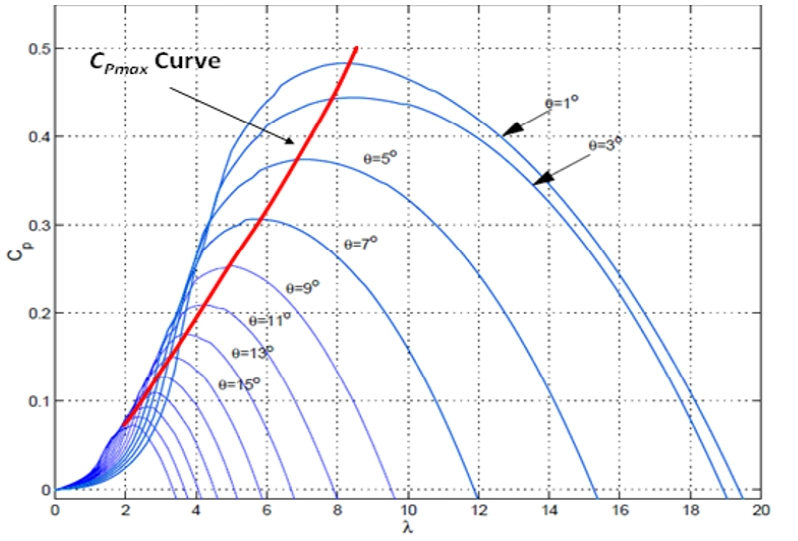
The aerodynamic heart of the model is the family of \(C_p\)-versus-\(\lambda\) curves, one for each pitch angle \(\beta\). Every curve has the same shape: \(C_p\) rises with \(\lambda\), reaches a peak, then falls away. So each curve has its own optimal tip-speed ratio. And when the pitch angle changes, the whole curve shifts — usually a larger pitch angle lowers the maximum achievable \(C_p\). In other words, pitch control reshapes the efficiency curve itself.

Power coefficient Cp against tip-speed ratio lambda for a family of blade pitch angles from about 1 to 15 degrees: each curve rises to a peak and falls away, higher pitch angles giving lower and earlier peaks, and a red locus line joins the peaks to mark the maximum-power-coefficient curve the controller aims for. — Figure 1 — The \(C_p\) curves: each pitch angle gives a curve that rises to a peak at an optimal tip-speed ratio and falls away. The locus of peaks marks \(C_{p,\max}\) — the best operating points the controller aims for.

Section 7

Why pitch angle matters

The pitch angle \(\beta\) changes the orientation of the blades relative to the wind, so pitching is a direct lever on aerodynamic capture. By pitching the blades the turbine can reduce the captured power, prevent over-power and regulate output above rated wind speed. Strictly, pitch is used mainly to limit captured power when needed: below rated wind speed the pitch is kept near its optimal value and speed control does the tracking, while above rated wind speed the pitch is increased to cut \(C_p\) and hold the power at rated.

Section 8

The unique optimal operating point

Because \(C_p\) as a function of \(\lambda\) has a single peak, a powerful conclusion follows: for a given wind speed and pitch angle there is one turbine rotational speed that achieves the maximum power coefficient \(C_{p,\max}\). Choose the right \(\omega_t\) and you get the right \(\lambda\), and the turbine sits at the top of its curve. The locus of those peaks, traced across wind conditions, is the line of best operating points — and it is exactly what the wind-turbine controller is trying to follow.

One best speed

For each wind speed there is a single rotor speed that maximises capture. Tracking it — keeping \(\lambda\) at \(\lambda_{opt}\) so \(C_p=C_{p,\max}\) — is the whole aim of wind MPPT.

Section 9

Below and above rated wind

The two control levers — rotor speed and pitch — are used in different wind regimes:

Table 2 — The two operating regimes and their control.
Regime	Wind Speed	Primary Control	Goal
Below rated	Below rated wind speed	Rotor speed (MPPT); pitch near optimal	Hold \(\lambda_{opt}\), maximise capture
Above rated	Above rated wind speed	Blade pitch	Reduce \(C_p\), limit power to rated

Below rated, the priority is efficiency, so the speed is moved to track the optimum; above rated, the priority is protection of the machine, so the pitch sheds the surplus aerodynamic power.

Section 10

Representing Cp as a polynomial

The real \(C_p\) surface comes from turbine design data, manufacturer data or look-up tables, but a model needs an expression it can evaluate quickly at every time-step. So the \(C_p\) curves are fitted with a high-order polynomial in \(\lambda\) and \(\beta\):

\[ C_p(\lambda,\beta) = \sum_{i=1}^{n}\sum_{j=1}^{n} a_{ij}\,\lambda^{i}\,\beta^{j} \]

\(a_{ij}\): fitted polynomial coefficients
\(\lambda,\beta\): tip-speed ratio and pitch angle
\(n\): polynomial order in each variable

The polynomial is just a practical way to reproduce the \(C_p\) surface as an analytical function, so the aerodynamic power can be computed continuously during simulation rather than interpolated from a table. It is only valid inside the range it was fitted for, though: the surface should be used within the turbine’s valid operating range, because extrapolating outside the fitted wind-speed, pitch or rotor-speed range can return non-physical \(C_p\) values.

Section 11

The aerodynamic model block

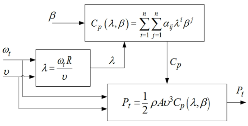
Assembled, the model is a short chain. Its inputs are the pitch angle \(\beta\), the turbine speed \(\omega_t\) and the wind speed \(v\). It first computes the tip-speed ratio \(\lambda = \omega_t R/v\); then the power coefficient \(C_p(\lambda,\beta)\) from the polynomial; then the mechanical power \(P_t = \tfrac{1}{2}\rho A v^3 C_p\). The mechanical torque follows directly from that power and the rotor speed, \(T_t = P_t/\omega_t\), so the same aerodynamic block also sets the torque applied to the drive-train model. That mechanical power and torque then drive the shaft and generator model, becoming the input to the electrical side.

Wind-turbine aerodynamic model block diagram: the turbine speed and wind speed form the tip-speed ratio lambda = omega_t R / v; lambda and the pitch angle beta feed a polynomial power-coefficient block Cp(lambda,beta); and Cp together with the air density, swept area and wind speed give the mechanical power P_t = one-half rho A v-cubed Cp. — Figure 2 — The aerodynamic model: wind speed, turbine speed and pitch in; tip-speed ratio and power coefficient computed; mechanical power \(P_t\) out, feeding the shaft and generator model.

What the mechanical power feeds into deserves a note, because the shaft is not rigid. In EMTP® the drive train is usually represented as a two-mass model: the rotor (blades and hub) with inertia \(J_t\) on one side, the generator with inertia \(J_g\) on the other, and a flexible shaft between them characterised by a torsional spring constant \(K_{tg}\) and a mutual damping \(D_{tg}\). The aerodynamic torque acts on \(J_t\); the electromagnetic torque acts on \(J_g\); and the shaft twists between them.

Why two masses, not one

A single lumped inertia would hide the drive-train’s fundamental torsional resonance — the mode in which the rotor and generator oscillate against each other through the compliant shaft. This lowest torsional mode is the one that matters for the electrical study, because control action and grid disturbances can excite it; the higher blade and shaft modes sit at much greater frequencies and carry far less energy, so retaining the two masses \(J_t\) and \(J_g\) with the shaft parameters \(K_{tg}\) and \(D_{tg}\) captures the behaviour that actually couples into the converter and the grid.

Section 12

From aerodynamics to the active-power reference

This aerodynamic model is what makes the turbine’s active-power reference meaningful: the reference is not arbitrary, it is rooted here. A small MPPT algorithm uses the \(C_p\) surface to find the optimal operating speed and generate the active-power reference for the electrical control. There is a clean special case worth knowing. If the turbine is held at the optimal tip-speed ratio, then \(v = \omega_t R/\lambda_{opt}\) and \(C_p = C_{p,\max}\); substituting into the power equation collapses everything onto the rotor speed:

\[ P_{t,\max} = K_{opt}\,\omega_t^{3}, \qquad K_{opt} = \tfrac{1}{2}\,\rho\,\pi R^{5}\,\frac{C_{p,\max}}{\lambda_{opt}^{3}} \]

\(P_{t,\max}\): captured power along the optimal locus
\(K_{opt}\): optimal-tracking gain (constant for a given turbine)
\(C_{p,\max},\lambda_{opt}\): peak power coefficient and the tip-speed ratio at which it occurs

Holding \(\lambda_{opt}\) as the wind varies makes the captured power follow \(\omega_t^3\) — which is why the wind MPPT reference so often appears as \(P_{ref}=K_{opt}\,\omega^3\). This cubic law only holds in the below-rated MPPT region, where the turbine is free to track \(\lambda_{opt}\); above rated wind speed the pitch control and power limiting take over and the reference is capped at rated. So the chain is: wind speed → aerodynamic model → best operating point → MPPT → active-power reference → converter control.

Section 13

Why wind is more involved than PV

It is worth contrasting this with the PV source. A PV array is a nonlinear source, but it has no rotating parts: its operating point is purely electrical. A wind turbine adds a mechanical world on top — the aerodynamic power depends on the wind, the rotor speed matters, the pitch matters, the \(C_p\) curves matter, and the shaft and gearbox dynamics and the generator interaction can matter too. So wind has a far stronger mechanical–electrical coupling than PV, which is exactly why its source model is more involved and why the MPPT problem is “operate at the best tip-speed ratio,” not simply “maximise electrical power.”

Section 14

Key points

Power from the wind, governed by the Cp surface

The wind, not the converter, creates the turbine’s power: the aerodynamic block is the mechanical source that feeds the generator and, through it, the electrical side.
The captured power \(P_t = \tfrac{1}{2}\rho A v^3 C_p\) varies with the cube of the wind speed, so it is very sensitive to the wind input.
The captured fraction \(C_p\) is not constant: it depends on the tip-speed ratio \(\lambda = \omega_t R/v\) and the pitch angle \(\beta\).
\(C_p\) peaks at an optimal \(\lambda\), so there is one best rotor speed for each wind — the aerodynamic basis of wind MPPT and the cubic reference \(P_{ref}=K_{opt}\,\omega^3\).
Above rated wind speed the blades pitch to reduce \(C_p\) and limit the power, protecting the machine.

For the rest of the chain, see the MPPT control, wind-park modelling and full-scale converter control guides.

References

EMTP® Documentation and Application Notes. Powersys / EMTP®.

Built on EMTP® · Expert spotlight

Henry Gras

Chief Operating Officer, PGSTech · Montréal, Canada

Henry Gras delivers the EMTP® University course “EMT Simulation and Analysis of Large-Scale Power Systems with Renewables” and works daily with the tool this article is written around.

Henry is based in Montréal, where he is Chief Operating Officer of PGSTech, the company responsible for EMTP® engineering services, commercialisation and continuing software development. He holds a master’s degree from Polytechnique Montréal, where he worked on electrical-machine research, and previously completed an engineering degree at École Centrale de Lyon in France.

Readers who want a structured programme on EMT simulation of large-scale power systems with renewables will find his EMTP® University course an excellent next step.

Henry’s technical expertise covers electromagnetic transient simulation, renewable-energy integration, power-system modelling, electrical machines, protection and specialist transient studies including TRV, transformer energisation, ferroresonance, insulation coordination and power quality.

Part 23 Reading now

Wind Turbine Aerodynamics and Power Coefficient

The power coefficient Cp, the tip-speed ratio, and the mechanical power source that drives the turbine model.

Series progress 23 of 30

Part 24

Variable-Speed Wind Turbine Control: MPPT and Pitch

Operating regions, the cubic MPPT law below rated, and pitch control above rated wind speed.