Renewable Modelling · Detailed & Average-Value Models

Detailed and Average-Value Converter Models in EMTP®

DM, AVM, PWM switching, timestep and model-selection limits

A converter controller produces one thing: a voltage reference. What a model does with that reference is the whole question here. A detailed model (DM) turns the reference into PWM gate pulses and explicit IGBT switching events, so the switched waveform and its harmonics are reproduced — at the cost of a very small timestep. An average-value model (AVM) applies the averaged converter voltage directly and removes the switching process, keeping the control, power-transfer and dc-link dynamics while dropping the switching ripple — far cheaper, and the default for most large EMT studies. Both represent the same converter; each is correct for a different study question.

Reading time ≈ 18 min · DM vs AVM, switching & timestep

A converter controller settles on a voltage reference; the model decides what becomes of it. Two standard representations answer that in different ways: the detailed model (DM) keeps the switches and the pulse-width modulation and turns the reference into real gate pulses, while the average-value model (AVM) replaces the switching bridge with an averaged controlled voltage source and imposes the commanded voltage directly. They model the same converter at two very different levels of electrical detail, and choosing between them is one of the routine judgements of EMT study work. As covered in the white-box / black-box guide, the electrical plant is usually built from standard EMT components; this page is about how much switching detail those components carry.

Abbreviations used on this page

DMDetailed model (explicit switching)

AVMAverage-value model

VSCVoltage-source converter

PWMPulse-width modulation

IGBTInsulated-gate bipolar transistor (the switch)

EMTElectromagnetic transient (simulation)

\(f_{sw}\)Switching (carrier) frequency

\(f_1\)Fundamental (grid) frequency

\(\Delta t\)Simulation timestep

\(V_{dc}\)dc-link voltage

FRTFault ride-through

SSCISub-synchronous control interaction

EMTP®Electromagnetic Transients Program

Key idea

The controller’s output is a voltage reference, not a switching command. How that reference becomes a converter voltage is what separates the two models — through real PWM pulses (DM) or as an averaged voltage applied directly (AVM).
A detailed model keeps every IGBT and the PWM, so the switched waveform and its switching-frequency harmonics are reproduced. It is the closest electrical picture of the hardware — but it forces \(\Delta t \ll T_{sw}\), and a timestep that is too large produces false, non-physical harmonics.
An average-value model replaces the switching bridge with an averaged controlled voltage source. It keeps the control, power-transfer, current-control and dc-link dynamics while dropping the switching ripple, so the timestep is no longer tied to \(f_{sw}\) — making it fast and scalable, and the default for most wind, PV and weak-grid studies.
Use DM when switching detail matters (harmonics, switching-frequency resonance, dc-side faults, high-frequency filter design); use AVM when control and system dynamics matter more. The detailed model is the benchmark that validates the average-value one.

Key terms used on this page

01Detailed model (DM)

A converter model with explicit IGBT switches and PWM gate signals, reproducing the switched waveform.

02Average-value model (AVM)

A model that replaces the switching bridge with an averaged controlled voltage source.

03Voltage reference

The desired converter terminal voltage produced by the controller — the converter’s actual input.

04PWM

Pulse-width modulation: compares the reference with a carrier to make gate signals for the switches.

05Two-level VSC

The classic three-phase, six-IGBT voltage-source converter shown in the detailed model.

06Switching frequency

The carrier rate \(f_{sw}\) at which the IGBTs switch; sets the harmonic spectrum and the timestep.

07Timestep

The EMT integration step \(\Delta t\); for a DM it must be far smaller than the switching period.

08False harmonics

Non-physical spectral content produced when a too-large timestep mis-samples switching instants.

09Modulation index

The normalised reference \(m\) that, with \(V_{dc}\), sets the averaged converter voltage.

10dc link

The capacitor (with measurement and chopper) joining the two converters of a back-to-back stage.

11Chopper

A braking branch across the dc link that dissipates surplus energy during disturbances.

12Benchmark validation

Using the detailed model as a reference to confirm the average-value model for the study of interest.

Section 1

Modelling the converter, not just its control

It is worth being clear about the distinction this page rests on. The earlier guides taught the control architecture — the PLL, the current loops, the sequence control, the FRT logic. This one is about the electrical model of the converter hardware. The two models here, DM and AVM, differ only in how the converter’s power stage is represented; the control wrapped around it can be identical. So the question is not “what does the controller do?” but “how faithfully are the switches and their waveform reproduced?”

Two levels of fidelity

DM captures the switching physics; AVM captures the averaged converter-control dynamics. Both are legitimate — the right one depends on what the study needs to see.

Section 2

The back-to-back converter and its dc link

The arrangement in question is a back-to-back converter: one VSC on one AC side, a second VSC on the other AC side, and a dc link in between. In the DFIG example the two sides are labelled the grid side and the rotor side, but the same modelling idea applies to any converter-interfaced wind or PV system, including the full-scale converter. The dc link itself carries the full electrical hardware: a capacitor, a dc-voltage measurement, and a chopper (braking) branch. Whichever fidelity you choose for the switching stage, this electrical skeleton stays the same.

Section 3

From a voltage reference to switching

One point is easy to miss and important to get right: the converter controller does not directly command IGBT switching. It produces a voltage reference — a desired AC voltage waveform, usually derived in the dq frame — and leaves the realisation to the power stage. What happens next is exactly where the two models differ. In a detailed model the PWM block compares that reference with a carrier and turns it into gate pulses, and the IGBTs physically realise the switching pattern. In an average-value model the averaged voltage is applied directly, with no gate pulses at all. The PWM is the bridge between a continuous desired voltage and the discrete switching behaviour of real semiconductors — a bridge the AVM simply skips.

The converter’s real input

Controller → voltage reference → PWM → gate signals → IGBTs. Where a model places itself on that chain — reproducing the pulses, or applying the averaged voltage directly — is the whole DM-versus-AVM question.

Section 4

Why switching produces harmonics

PWM does not produce a single clean sinusoid. Because the output is built by rapidly connecting semiconductor states rather than by an ideal analogue source, the converter voltage is a switched waveform, and its spectrum spreads into components clustered around the switching carrier and its sidebands. It contains the desired fundamental plus content at the switching frequency and sidebands around it:

\[ f_h = k\,f_{sw} \pm n\,f_1, \qquad k = 1,2,3,\dots,\ \ n = 0,1,2,\dots \]

\(f_h\): frequencies present in the switched converter voltage
\(f_{sw}\): switching (carrier) frequency
\(f_1\): fundamental (grid) frequency
\(k,\ n\): carrier multiple and sideband order

The spectrum clusters in sidebands around the carrier and its multiples. Resolving that content is why a switched converter needs filter inductors, sometimes harmonic filters, and a careful timestep — and reproducing it explicitly is exactly what the detailed model does.

Section 5

The Detailed Model (DM)

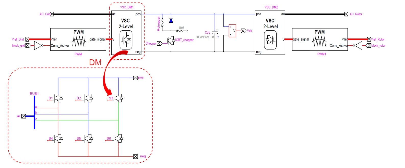
The detailed model represents a two-level VSC with its six switches — the classic three-phase, two-level voltage-source converter. Every IGBT is represented explicitly, the switching states are modelled, the PWM produces real gate pulses, and the converter waveform includes the switching effects. It is the closest electrical representation of the switching bridge — but that closeness is only realised if the timestep, the device model and the controls are suitable; its accuracy depends strongly on the timestep and on how well the switching events are resolved.

Detailed model of a back-to-back two-level voltage-source converter in EMTP: the grid-side and rotor-side VSC bridges with their PWM blocks, the dc-link capacitor and chopper, and one bridge expanded to show the six explicit IGBTs S1 to S6 switched by the PWM gate signals. — Figure 1 — The detailed model of a two-level VSC: six explicit IGBTs switched by PWM gate pulses, reproducing the real switched voltage waveform and its switching-frequency harmonics.

Section 6

Why the Detailed Model is expensive

The cost of that fidelity is the timestep. To simulate switching explicitly, the EMT timestep must be much smaller than the switching period, so that the switching instants align properly with the simulation mesh:

\[ \Delta t \ll T_{sw} = \frac{1}{f_{sw}}, \qquad \Delta t \lesssim \frac{T_{sw}}{N}, \quad N \sim 20\text{–}100 \]

\(\Delta t\): EMT simulation timestep
\(T_{sw}\): switching period
\(f_{sw}\): switching frequency
\(N\): samples wanted per switching period

A converter switching at a few kHz typically needs a timestep of microseconds or below — but there is no single universal value. The step has to be chosen against the switching frequency and the study objective, and it also depends on the converter topology, the filters and the frequency range of interest. Whatever the value, a small step becomes costly when many converters, a large grid model or a long simulation window are involved — so the detailed model is faithful, but expensive.

Section 7

False harmonics from a too-large timestep

This is the practical warning that matters most. A timestep that is too large relative to the switching frequency does not simply make the model less accurate — it mis-samples the switching events and can create harmonic content that is not physical, the wrong dc-link ripple and misleading current waveforms. A poor timestep choice does not just make a detailed model coarse; it can make it misleading. That is why detailed converter modelling has to be done carefully, with the timestep chosen against the switching frequency rather than out of habit.

The detailed-model timestep trap

A timestep that is too large for \(f_{sw}\) mis-samples the switching instants and injects non-physical harmonics.
The dc-link ripple and the current-waveform shape come out wrong, so the model looks detailed but is not trustworthy.
The fix is not a bigger model — it is a smaller timestep, or moving to an average-value model where switching is not resolved at all.

Section 8

The Average-Value Model (AVM)

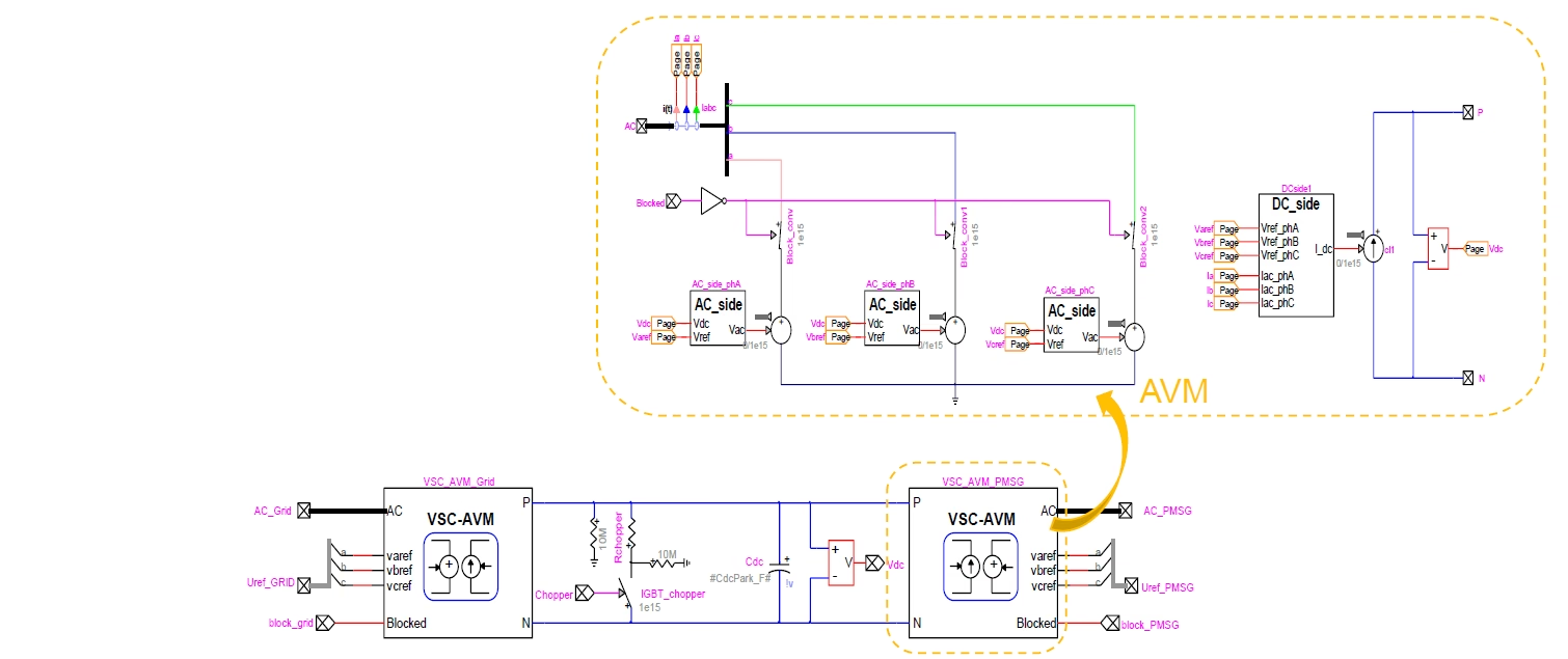
The average-value model takes a different route. Rather than removing the switches and leaving a bare voltage source, it replaces the switching bridge with a power-consistent controlled-source representation: a controlled voltage source on the AC side driven by the controller’s modulation command, with the dc side following from power balance. The pulse-by-pulse switching is dropped, but the averaged AC/DC power transfer, the current-control dynamics, the dc-link behaviour and the outer control response are all preserved. The AVM must keep the AC and DC sides energetically consistent — otherwise it would be only a voltage source, not a converter model — so it imposes the commanded averaged voltage and conserves power on the dc side:

\[ \bar{v}_{\mathrm{conv},abc} = m_{abc}\,\frac{V_{dc}}{2}, \qquad V_{dc}\,i_{dc} = \tfrac{3}{2}\big(v_d i_d + v_q i_q\big) \]

\(\bar{v}_{\mathrm{conv},abc}\): averaged converter terminal voltage applied to the AC side
\(m_{abc}\): modulation functions from the controller’s voltage reference
\(V_{dc}\): dc-link voltage
\(i_{dc}\): averaged dc-side current (from AC-side power)

The converter is treated as if it can realise the commanded AC voltage without explicit switching pulses, while the dc current follows from power balance. No gate signals, no carrier — and no switching events for the solver to resolve. This is the high-level idea; how the controlled AC-side sources and the dc-side current source are actually built is developed in the AVM principles guide.

Average-value model of a back-to-back converter in EMTP: the grid-side and machine-side VSC-AVM bridges, with the switching stage expanded into averaged controlled AC-side voltage sources and a dc-side current source, so no IGBTs are switched and the commanded voltage is applied directly. — Figure 2 — The average-value model: the switching bridge is replaced by averaged controlled voltage sources, so the commanded voltage is applied directly with no PWM pulses, while dc-side power balance is preserved.

Section 9

What “average value” really means

Physically, an AVM keeps the fundamental dynamic effect of the converter while discarding the detailed switching ripple. It preserves the control behaviour, the power-transfer dynamics, the current-control response, the dc-link behaviour and the interaction with the network at EMT control timescales. What it does not preserve is the exact switching waveform, the detailed PWM harmonics and the pulse-by-pulse semiconductor behaviour. In short, the AVM is control-faithful but switching-simplified — and that is a deliberate choice, not a defect.

Section 10

Why AVM is the workhorse

For most power-system EMT studies the quantities of interest are faults, voltage dips, current control, fault ride-through, dc-link regulation, weak-grid interaction, plant-controller response and stability — not every switching edge or PWM harmonic. The AVM delivers those dynamics without forcing an extremely small timestep, which is the heart of its appeal:

The timestep is no longer dictated by the switching frequency, because there are no switching events to resolve.
Simulations run faster and are numerically easier, which matters for long windows and many converters.
The model scales to large networks, sensitivity scans and full wind-farm or PV-plant studies.
Initialisation is generally easier than for a fully switched model.

That combination is why the AVM is the default choice for wind-farm and PV-plant EMT studies, weak-grid work, controller tuning and FRT studies, and large network-interaction analyses.

How large the saving actually is

The gain is not marginal. In a published two-level VSC comparison the average-value model reproduces the detailed model’s response closely even at a coarse 50 μs step, whereas the detailed model needs a step near 10 μs to resolve its switching — and for that case the AVM runs well over nine times faster in CPU time. That figure is specific to the case, but the general engineering point holds regardless: because the AVM does not resolve switching events, its timestep is not tied to the switching frequency, so it scales to full plant studies while the detailed model is reserved for switching-level questions.

Section 11

What AVM cannot do well

The dividing line is simple. An AVM is suitable when the study concerns system-level dynamics: controller response, fault ride-through, weak-grid interaction, dc-link regulation, plant-level EMT behaviour and stability — including SSCI and weak-grid work, provided the frequencies that matter sit below the switching detail it omits. A DM is needed when the switching process itself is the subject: PWM harmonics, switching-frequency resonance, converter-side filter design at high frequency, semiconductor stress and switching-sequence effects, and some dc-side fault behaviour. If the switching process itself matters, the average-value model is not enough.

Section 12

Choosing between DM and AVM

The decision comes down to whether the study needs switching detail or system and control dynamics. Put side by side:

Table 1 — Detailed model and average-value model compared.
Aspect	Detailed Model (DM)	Average-Value Model (AVM)
Switching detail	Every IGBT and PWM pulse explicit	Bridge replaced by an averaged controlled source
Timestep	\(\Delta t \ll T_{sw}\) — microseconds	Free of \(f_{sw}\); larger steps allowed
Harmonics	Switching harmonics reproduced	Switching harmonics not represented
dc-link behaviour	Ripple resolved pulse by pulse	Averaged; dc current from power balance
Control response	Preserved	Preserved
Study size	Small — high cost per converter	Large — fast and scalable
Best use	Harmonics, switching resonance, dc-side faults, filter design	Control, FRT, weak-grid, stability, plant-level studies
Main limitation	Tiny timestep; false harmonics if mis-set	No switching detail or switching-frequency phenomena

In practice the choice is made on the study objective:

Reach for AVM when you care about controller response, FRT, weak-grid stability, plant interaction, dc-link control, large EMT network studies, initialisation efficiency or runtime.
Reach for DM when you care about PWM harmonics, switching-frequency effects, converter waveform detail, dc-side switching stress, semiconductor-level behaviour or high-frequency filter validation.

Section 13

Using the Detailed Model to validate the AVM

The two models are not rivals so much as a benchmark and a workhorse. A common and sound workflow is to build or trust the detailed model, compare it against the average-value model, and confirm that for the phenomena of interest — currents, power, dc voltage, control response, fault response — the two are close enough. Once the AVM is validated against the DM for those quantities, it can be used with confidence for faster studies, bigger grids and sensitivity scans, while the detailed model is kept in reserve for the questions that genuinely need switching detail.

Benchmark, then scale

Validate the AVM against the DM for the responses that matter; then run the AVM for the large, fast, repeated studies, and return to the DM only for switching-level questions.

Section 14

Key points

Same converter, two fidelities — chosen by the study

DM resolves PWM and switching. Every IGBT and PWM pulse is explicit, reproducing the switched waveform and its switching-frequency harmonics.
AVM applies the averaged converter voltage. A power-consistent controlled source imposes the commanded voltage directly and conserves dc-side power, keeping the control and dc-link dynamics without switching ripple.
DM needs a small timestep. \(\Delta t \ll T_{sw}\), so a detailed model is expensive; an AVM is free of the switching frequency and far faster.
A poor timestep creates false harmonics. Too large a step mis-samples the switching instants and produces non-physical harmonics, the wrong dc-link ripple and misleading currents.
AVM is preferred for large system and control studies — unless switching detail is the subject (harmonics, switching resonance, dc-side faults, filter design), where a DM is required; validate the AVM against the DM before trusting it at scale.

For the control that wraps the converter and the model-transparency question, see the DFIG converter control, full-scale converter control and white-box / black-box guides.

References

EMTP® Documentation and Application Notes. Powersys / EMTP®.

Built on EMTP® · Expert spotlight

Henry Gras

Chief Operating Officer, PGSTech · Montréal, Canada

Henry Gras delivers the EMTP® University course “EMT Simulation and Analysis of Large-Scale Power Systems with Renewables” and works daily with the tool this article is written around.

Henry is based in Montréal, where he is Chief Operating Officer of PGSTech, the company responsible for EMTP® engineering services, commercialisation and continuing software development. He holds a master’s degree from Polytechnique Montréal, where he worked on electrical-machine research, and previously completed an engineering degree at École Centrale de Lyon in France.

Readers who want a structured programme on EMT simulation of large-scale power systems with renewables will find his EMTP® University course an excellent next step.

Henry’s technical expertise covers electromagnetic transient simulation, renewable-energy integration, power-system modelling, electrical machines, protection and specialist transient studies including TRV, transformer energisation, ferroresonance, insulation coordination and power quality.

Part 18 Reading now

Detailed and Average-Value Converter Models

Detailed switching models versus average-value models: accuracy, timestep and when each one is appropriate.

Series progress 18 of 30

Part 19

AVM Principles: the Controlled-Source Model

Building the average-value converter from controlled sources that reproduce the fundamental behaviour without switching.