EMT Modelling · Load-Flow Initialisation

Synchronous-Machine Load-Flow Initialisation in EMTP®: The Example and the Study Workflow

An electromagnetic-transient model only tells the truth if it starts from the truth. It is not enough to know the right bus voltage and power — every internal state of every dynamic device must begin in equilibrium, or the first seconds of the run fill with artificial transients. The synchronous machine (SM) makes this concrete: its rotor angle, field excitation and controller states must all be set from a solved operating point. This guide uses that example to explain why load-flow initialisation matters, how EMTP® (the Electromagnetic Transients Program) back-initialises a machine and its automatic voltage regulator (AVR) and governor, and how the same philosophy carries through to converter plants, imported cases and the choice of study mode.

Reading time ≈ 26 min · SM initialisation & EMTP® study workflow

Run a detailed electromagnetic-transient (EMT) model and the way it starts matters more than it first appears: poor initialisation can contaminate the early results and can sometimes destabilise the whole run, so the pre-event period has to be checked before any post-event result is trusted. If the model is started from a state that is not in equilibrium, the first seconds fill with a transient that has nothing to do with the event you set out to study — a numerical initialisation artefact, not a physical event in the network — while the machine searches for its operating point and currents, torques and control outputs swing. The fix is to start from a solved steady state, and not only of the network: every internal state of every dynamic device must begin in balance. The synchronous machine is the clearest way to see why, so this guide opens with it, then carries the same idea through to converter plants, imported cases and the choice of study mode. It is the companion to the wind-park load-flow and initialisation arrangement.
Abbreviations used on this page
EMTElectromagnetic transient (time domain)
EMTP®Electromagnetic Transients Program
SMSynchronous machine
AVRAutomatic voltage regulator (excitation control)
PV / PQVoltage-controlled / power-controlled bus
PLLPhase-locked loop (converter synchronisation)
SEXSSimplified excitation-system (exciter) model
emfElectromotive force (machine internal voltage)
\(\delta\)Rotor (load) angle
\(X_d\)Machine reactance (here the synchronous reactance)
PWMPulse-width modulation (converter switching)
PSS/ESiemens PTI power-system simulator (another tool)
Key idea
  1. A correct EMT run must start from the steady state of both the network and every internal dynamic state. The load flow supplies the network anchor; EMTP® back-initialises the machine and its controllers from it.
  2. For a synchronous machine, two conditions must be matched: the rotor angle (for active power, across transformer phase shifts) and the field/excitation (for terminal voltage and reactive power). Guessing both by hand across a real network is unreliable.
  3. Controllers carry memory. A well-built model has an explicit initialisation path (e.g. a SEXS exciter with a hold block) that computes the steady reference before the dynamics run — so the trace starts flat instead of ramping.
  4. The philosophy scales: synchronous machines initialise directly; converter plants settle behind a temporary ideal source. Imported (PSS/E) cases are re-solved in EMTP® to validate them, generators keep PV/PQ enforcement, and one model adapts its internal form to load-flow, EMT or harmonic studies.
Key terms used on this page
01Operating point
The consistent steady state (voltages, currents, powers, internal states) the model must begin from.
02Load-flow initialisation
Using the solved load flow to set every dynamic device’s internal states so the run starts in balance.
03Rotor (load) angle
The angle between the machine’s internal emf and the network voltage; it sets the active power.
04Field / excitation voltage
The dc field input that sets the internal emf and so the terminal voltage and reactive power.
05Power-angle relationship
Active power varies as \(\sin\delta\); a wrong angle gives the wrong power and a rotor swing.
06AVR / governor
Excitation and speed controllers; their internal states must be initialised, not started at zero.
07Controller memory
The internal state of a transfer function (integrator, lag); a wrong start makes the output ramp.
08Initialisation vs dynamics
A model structure that computes a steady reference first, then runs the time-domain transfer functions.
09Ideal initialisation source
A temporary source that holds the correct terminal condition while a converter plant settles internally.
10PV / PQ enforcement
A generator holds P and V until a reactive limit is hit, then switches to fixed P and Q.
11Wrong equilibrium
A non-linear system can settle to an unintended operating branch if the initial guess is poor.
12Multi-study model
One device whose internal representation changes with the study: load flow, EMT, or harmonic scan.

Section 1

Initialisation is more than bus voltage and power

It is tempting to think that knowing the bus voltage and the injected power is enough to start a simulation. For a static calculation it is. For a dynamic model it is not, because the model also carries internal states that the terminal quantities alone do not pin down. The general EMT truth is simple to state: a time-domain run must begin from the steady state of both the network and the internal models. Miss the second half and the model is internally inconsistent at \(t=0\); it will spend real simulation time settling, and that settling is pure artefact.

The synchronous machine is the ideal example because the problem is obvious and the physics is familiar. The same lesson then transfers, with more difficulty, to converter-based plants — which is exactly why EMTP® treats their initialisation with extra care.

The principle

For the synchronous machine this has a concrete meaning: matching the terminal voltage and power is not enough — the rotor angle and the field behind them must also be set from the load flow. The sections that follow show why those two quantities matter, and how EMTP® back-initialises them.

Section 2

Why a synchronous machine will not start from nothing

A synchronous machine is not a P–Q box. “Every internal dynamic state” is concrete here: for a synchronous machine it means all of the following, which must be mutually consistent for the machine to sit still:

  • the rotor angle and rotor speed;
  • the stator and rotor flux — the machine’s magnetic state;
  • the field / excitation voltage;
  • the exciter / automatic voltage regulator (AVR) internal states;
  • the governor and turbine states, and the mechanical power;
  • any controller integrator states in the excitation and speed loops.

Start any of these at the wrong value and the machine is not in equilibrium. Electrical torque no longer balances mechanical torque, and the rotor begins to accelerate or decelerate — the machine literally searches for its operating point through an electromechanical oscillation. Two matching conditions matter most: the rotor angle must align correctly with the electrical angle (for active power), and the field must be correct (for reactive power and terminal voltage). The next sections take these in turn.

Section 3

Rotor angle sets the active power

A synchronous machine delivers active power according to the angular relationship between its internal emf and the network voltage. The classic simplified power-angle relationship — an explanatory picture, not the full set of machine equations EMTP® actually solves — has the power varying with the sine of that angle:

\[ P = \frac{E_q\,V}{X_d}\,\sin\delta \]
\(P\)
active power delivered to the network
\(E_q\)
machine internal emf (set by the field/excitation)
\(V\)
network (terminal) voltage magnitude
\(X_d\)
the machine’s synchronous reactance — a single simplified reactance between the internal emf and the network for this steady-state relationship (not the transient reactance \(X'_d\), which belongs to fast-transient analysis)
\(\delta\)
the rotor/load angle between the internal emf and the network voltage, measured in the network voltage reference frame

Guess \(\delta\) wrongly and the machine produces the wrong active power at \(t=0\): electrical torque no longer matches mechanical torque, the rotor swings, the power oscillates, and the AVR and governor react — a transient that is entirely a start-up artefact.

This is why the initial angle cannot be treated casually. A small error in \(\delta\) is a real mismatch in torque, and the machine will take time to swing into the correct angle — time the study wastes before the event of interest even begins.

Section 4

Transformer phase shift and the angle guess

Guessing the machine-side angle from the network side is harder than it looks, because transformers rotate the phase. A transformer’s vector group (for example a delta–wye connection) introduces a fixed phase shift — commonly \(30^\circ\) — between the voltages on its two sides, and a dedicated phase-shifting transformer adds a further, adjustable shift. Each of these changes the relationship between the generator terminal angle and the remote grid reference angle, so reconstructing the machine terminal angle by hand would mean accounting for every such shift between the machine and the bus whose angle you think you know, while simultaneously satisfying the required power transfer.

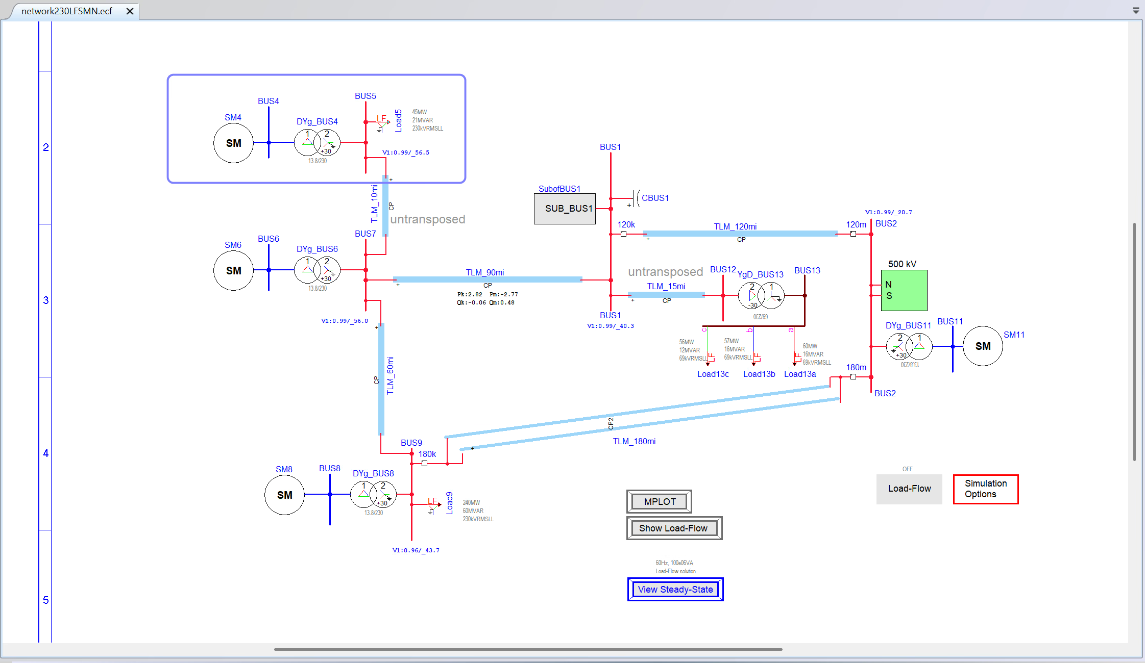
Single-line diagram: synchronous machine SM4 behind a delta-wye (DYg) step-up transformer, 13.8 / 230 kV, feeding the network bus and load.
Figure 1 — The synchronous machine SM4 behind a delta–wye (DYg) step-up transformer, 13.8 / 230 kV, feeding the network and load. The transformer’s \(+30^\circ\) phase shift is exactly the kind of offset that makes the machine-side angle awkward to guess by hand; a solved load flow accounts for it automatically.

In a tiny textbook case you might manage it by inspection, perhaps reading a \(+30^\circ\) hint straight off the transformer and assuming the machine angle is near it. In a real network, with several transformers, lines and loads, hand-reconstruction is impractical and unreliable. The point is not that it is impossible — it is that it is the wrong way to work when a load-flow solver will give the exact answer.

Section 5

Field voltage sets the reactive power

Matching the angle fixes the active power, but it says little about reactive power. For a synchronous machine, reactive output is governed by excitation: raise the field and the machine over-excites and exports reactive power; lower it and the machine under-excites and may absorb reactive power or fail to support its bus. In the same simplified picture, the reactive power is:

\[ Q = \frac{E_q\,V\cos\delta - V^{2}}{X_d} \]
\(Q\)
reactive power delivered to the network
\(E_q\)
internal emf, raised or lowered by the field voltage
\(V\)
network (terminal) voltage magnitude
\(X_d\)
the machine’s synchronous reactance (the same simplified reactance as above)
\(\delta\)
the rotor/load angle

With the angle already fixed for active power, \(Q\) is driven mainly by \(E_q\) — that is, by the field. Excitation therefore strongly influences the terminal voltage and reactive power, but the exact result depends on the network, the machine model, the AVR settings and limits, and the operating point; this simplified expression only shows the direction of the effect. Even a correct angle is not enough: the excitation state must also be right.

There are therefore two steady-state conditions to satisfy at once: the rotor angle for the active-power balance, and the field/excitation for the voltage–reactive balance. Both come out of a load-flow solution; neither is reliable to guess.

Section 6

Controllers carry memory too

Even if the machine’s electromagnetic and mechanical states were perfect, the controllers would still need attention. Two separate paths matter here: the AVR / excitation path, which acts mainly on terminal voltage, reactive power and field voltage; and the governor / turbine path, which acts mainly on mechanical power, speed and frequency response. Each is built from transfer functions — integrators, lag–lead blocks, PI loops — and a transfer function has internal memory. If a block should be sitting at some steady output but its internal state is initialised at zero, then at \(t=0\) its output is wrong and the controller must move toward the correct value — another artificial transient, layered on top of any machine mismatch.

With a load-flow solution in hand, EMTP® works step by step through the transfer functions and sets each one consistently, so no controller block has to ramp from zero when the run begins.

Section 7

Inside a well-built model: initialisation versus dynamics

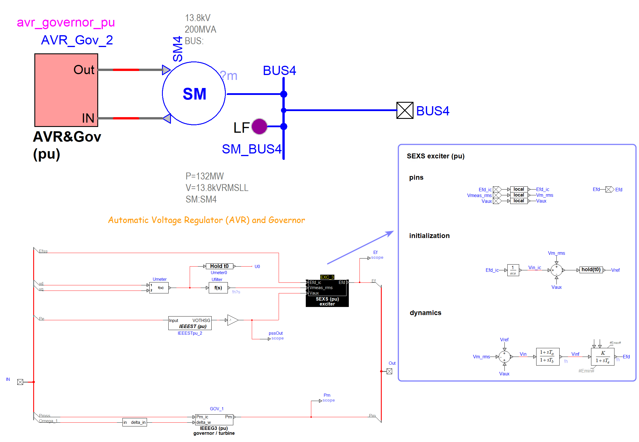
A properly written dynamic model makes this explicit by separating two paths. An initialisation path computes the steady-state reference the model should hold at \(t=0\); a dynamics path then runs the actual transfer functions starting from that consistent point. The simplified excitation-system (SEXS) model — one simple, standard AVR model, used here only as an example of how any controller is initialised, not as the sole choice — shows the pattern clearly: input/output pins, an initialisation section that derives the steady reference and captures it in a hold block, and a separate dynamics section with the lag–lead and gain/lag transfer functions that run during the simulation. The hold block is the key: during initialisation it holds (injects) the calculated steady-state controller output, so when the run starts the dynamic path begins from that correct value instead of ramping up from zero.

A SEXS exciter controller model with a separate initialisation path (computing the steady reference and holding it via a hold block) and a dynamics path of lag-lead and gain/lag transfer functions that run during the simulation.
Figure 2 — A well-built controller model separates an initialisation path — which computes the steady reference and holds it (here via a hold(t0) block) — from the dynamics path of transfer functions that run during the simulation. The same initialisation-versus-dynamics split applies to the governor and to any other controller carrying internal memory. Initialising the dynamic states from the held reference is what stops the output ramping at \(t=0\).

For the user this is invisible: the finished model simply starts correctly. For the developer it is real work, because each block must be initialised consistently with the block that follows it — tracing backward from the load-flow terminal conditions to the internal references, controller outputs and transfer-function states. That backward chain is the price of a model that starts in equilibrium, and it is why the explicit initialisation section exists.

Section 8

What a bad initial guess costs

Start from a non-equilibrium state and the system performs a genuine transient — just not one you care about. In a synchronous-machine network that start-up transient can involve rotor-angle swing, power oscillation, excitation movement, governor action, voltage adjustment and interaction with loads and lines. The network is not wrong; the initial state is. A reasonable guess might still take several seconds to settle; a poor guess can take the best part of ten seconds, and can do something worse.

Non-linear systems can have more than one equilibrium or more than one numerically reachable operating branch. If the initial guess is poor, the time-domain dynamics may settle toward a state that is not the intended operating point — the wrong reactive output, the wrong machine angle, a different internal-state combination, or in a bad case an unstable or unacceptable condition. This is precisely why a time-domain run is not a substitute for load-flow initialisation: settling is not guaranteed to land where you wanted.

Avoid these
  • Energising a dynamic model from an arbitrary or zero state and treating the start-up swing as physical.
  • Hand-guessing machine angles across transformer phase shifts in anything but a trivial case.
  • Setting the field/excitation by feel — the terminal voltage and reactive power will be wrong.
  • Leaving controller (AVR/governor) states at zero so their outputs ramp at \(t=0\).
  • Trusting that a time-domain run will “settle to the right answer” — it may settle to a different equilibrium.
  • Applying the studied disturbance before the model has reached its operating point.

Section 9

What the load flow provides

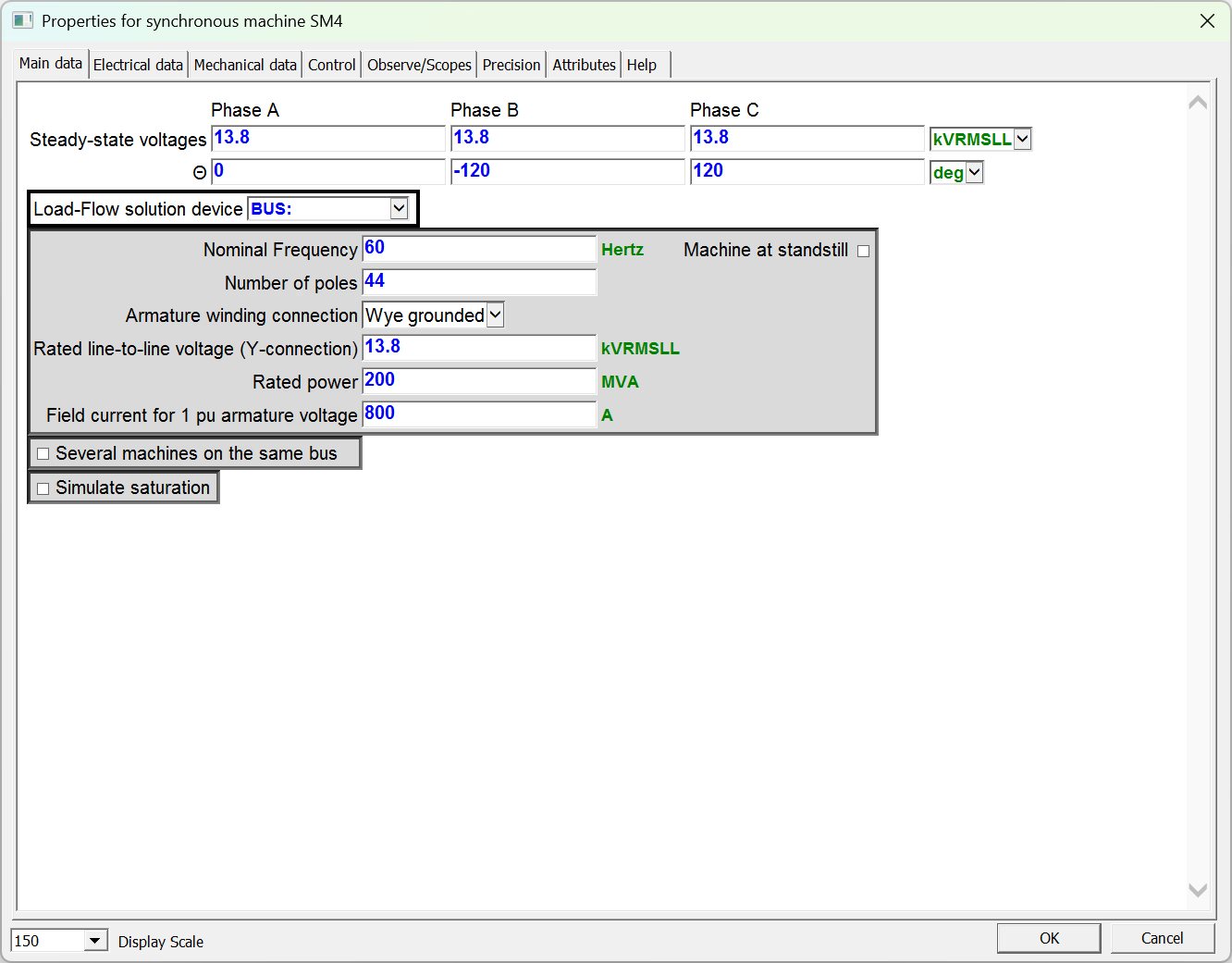
Once EMTP® solves the load flow it knows the voltage magnitude and angle at every bus, the active and reactive injections, the network currents and the flows through transformers and lines. From that solved operating point it can infer, for each machine, the steady-state quantities its dynamic model needs — the correct terminal voltage and the internal condition consistent with the given active and reactive output. The machine is, in effect, linked to its solved bus.

Synchronous-machine data page referencing a load-flow solution device (the bus) alongside the steady-state voltages and ratings, so the machine's internal initialisation is taken from the solved operating point.
Figure 3 — The synchronous-machine data page references a load-flow solution device (the bus) alongside its steady-state voltages and ratings, so the machine’s internal initialisation — its rotor angle and speed, the stator and rotor fluxes and the field voltage, together with the AVR and governor controller memory — is taken directly from the solved load-flow operating point rather than guessed, and the machine is handed to the time-domain solution already in equilibrium.

So the load flow is not merely a network solution; it is the anchor for initialising the machine model itself. The angle that balances the active power and the excitation that produces the right reactive power both fall out of it, automatically and consistently. And because EMTP® can represent phase-domain network conditions where the model and data support it, the resulting operating point can be richer than a single positive-sequence voltage magnitude and angle. None of this removes the need for sound inputs, though: correct machine parameters, saturation treatment, controller settings and limits, transformer connections, and a converged load-flow result are all required for the initialisation to be right.

Section 10

The flat trace: the proof it worked

Run the same case with load-flow initialisation and the trace starts flat. Concretely, before any disturbance the terminal voltage, the active and reactive power, the stator current, the rotor speed, the mechanical power, the field voltage and the AVR / governor outputs should all sit steady, with no drift or swing. That flatness is the proof: the machine is already at equilibrium, its controllers are already at their steady operating points, and the bus voltage and angle are already correct, so no start-up correction is needed. When a real event happens later — a capacitor-bank energisation, but equally a fault, a switching event, a control step, a motor start, a line energisation or a renewable-plant disturbance — the transient you observe is the one you actually care about.

That is the whole purpose of initialisation: remove the fake start-up transients so that only the real study transients remain. It matters even more in large or weak grids, where you cannot afford to simulate ten useless seconds before the disturbance, the timestep is small and the states are many, and where a start-up transient can interact with weak-grid devices, renewable controls or protection and make the run fail or mislead.

Flat is good

A flat pre-event trace is the quickest visual check that initialisation succeeded. If the waveforms drift or swing before any disturbance is applied, the model was not started at its operating point.

A short routine makes the check systematic:

  • run the case with no disturbance first, and confirm the pre-event traces are flat;
  • check the load-flow mismatch is negligible;
  • check the machine \(P\), \(Q\) and \(V\) against the load-flow solution;
  • check the rotor speed is steady and the field voltage sits at its expected value;
  • check the AVR and governor outputs are steady, not ramping;
  • only then apply the actual disturbance, once the model is settled.

Section 11

From synchronous machines to converter plants

Wind and PV plants need the same thing for the same reason — but the implementation differs. A synchronous machine can be initialised directly at the first time step, because its required internal state follows cleanly from the load-flow terminal conditions. A converter-based plant is harder: it has many tightly coupled internal states — phase-locked-loop (PLL) phase and filtering, inner current loops, the dc-link behaviour, outer voltage/reactive loops, plant-controller states, limiters and measurement delays — and obtaining an exactly consistent value for every one of them at the very first step is not yet as clean as for a classical machine.

So EMTP® holds the correct terminal condition with a temporary ideal voltage source while the plant settles behind it, then releases the source once the internal states have converged. The detailed switch arrangement, the length of that settling window and the source behaviour are wind/PV-specific and are covered on the dedicated wind-park load-flow and initialisation guide (and the PV-park modelling page) — they are not repeated here. The essential contrast is all this page needs: a synchronous machine reaches its operating point directly, while a converter plant is given a brief, isolated window to get there.

Same philosophy, different mechanism

Hold the correct operating point while the internal model settles, then release it. The synchronous machine reaches the point instantly; the converter plant is given a brief, isolated window to get there.

Section 12

Importing a case — and re-solving it

Cases often arrive from another tool. A network from PSS/E (Siemens PTI’s power-system simulator) — its raw data, sequence data and available dynamic data — can be imported into EMTP®, but the imported solution is not trusted blindly. EMTP® rebuilds the network in its own representation and runs its own load flow, then compares the result with the source case. This does two jobs at once.

  • It validates the import. Cross-tool transfers can introduce small mismatches — unit conventions, transformer modelling, bus-type interpretation, control limits, shunt signs, phase-shift handling, missing or estimated data, unsupported user-defined pieces. If the EMTP® load flow matches the source closely, the import is sound; if not, something needs attention.
  • It produces EMTP®’s own operating point. The dynamic initialisation must be consistent with the network as built inside EMTP®, so the program needs a solution in its own formulation — the source result is a benchmark, not the starting state.

One caveat is worth stating plainly: standard, supported models import systematically, but arbitrary user-defined dynamic models are not guaranteed to transfer automatically. Such models embed assumptions about one tool’s internal interface, so unless a dedicated translator exists, some manual engineering is needed to bring them across. That is normal for any cross-tool migration.

Section 13

Automatic PV/PQ enforcement

In load flow a generator is more than a machine block: it also carries an operating rule. The robust approach — preserved on import — is to attach the generator’s load-flow enforcement device with its control voltage, control power and reactive limits, so the imported case keeps the same generator behaviour it had in the source tool. The behaviour itself is the familiar PV/PQ switch: the unit runs as a PV (voltage-controlled) bus, holding \(P\) and \(V\), until it reaches a reactive limit and reverts to a PQ (power-controlled) bus, holding \(P\) and \(Q\).

Table 1 — How a generator is represented in load flow, and when it switches from PV to PQ.
Bus TypeHeld FixedFree to AdjustRole / Switch Condition
PV busActive power \(P\) and voltage magnitude \(V\)Reactive power \(Q\), within the machine’s limitsNormal mode while \(Q\) stays inside the reactive capability.
PQ busActive power \(P\) and reactive power \(Q\) (held at the limit)Voltage \(V\) (no longer controlled by this unit)Taken up automatically when the machine hits a reactive limit and can no longer hold \(V\).

Preserving this PV→PQ logic matters: drop it and the imported case can solve to a different operating point than the source, and the dynamic initialisation would then start from the wrong place. One detail to get right is the reactive-limit sign convention: the \(Q\) limits should follow the project or tool convention — positive \(Q\) may mean reactive power injected or absorbed depending on that convention — so the sign of \(Q\) must never be left ambiguous.

Section 14

One model, many study modes

A particularly useful idea is that a single plant device need not use the same internal representation for every study. Set it for time-domain work and all the dynamic parts are present; switch it to a harmonic or frequency-scan study and some dynamic parts are excluded and replaced by other representations, such as harmonic sources. The top-level device stays the same; its internals adapt to the question.

Table 2 — One plant device, three internal representations selected by the study.
StudyInternal RepresentationWhat It Captures
Load flow (steady state)PV/PQ equivalent plus initialisation logicThe operating point that seeds every dynamic state.
Time-domain EMTFull dynamic model — machine/converter, controls, protectionSwitching and control dynamics, faults and transients.
Harmonic / frequency scanHarmonic sources with the passive network; dynamic loops excludedFrequency-domain response and resonances.

The practical payoff is that one organised device, with its data in one place, can serve load flow, steady-state initialisation, time-domain EMT and harmonic studies — instead of maintaining several separate, drifting versions. It helps that EMTP® keeps its scripts and models open: advanced users can inspect how the steady-state, load-flow and time-domain parts are linked, customise libraries, and drop in manufacturer or user blocks where the standard library is not enough.

Section 15

When can you trust harmonic results?

The flip side of the multi-study idea is a caution worth keeping. A model that is fine for load flow or EMT control-response studies is not automatically suitable for harmonic-emission work unless its harmonic source and impedance representation are appropriate. To give realistic harmonic results, a converter-based model must actually be detailed enough to produce harmonics: a proper pulse-width-modulation (PWM) representation, accurate device characteristics, appropriate delays, accurate measurement and filter dynamics, sufficient inner- and outer-loop detail, and a very small time step. A model built for grid-code fault response or electromechanical transients may simply not contain the switching detail that harmonics come from.

So the honest question to ask of any converter model is: what was it built for? A model designed for dynamic response is not automatically a harmonic model, and using it as one will give confident but wrong numbers. Match the model’s fidelity to the study, exactly as you match the initialisation to the dynamics.

Section 16

Key points

The load-flow result is the machine’s starting operating point

The load-flow result is not just a network solution; it is the operating point used to initialise the machine and its controllers. For a synchronous machine the key states are the rotor angle, the speed, the excitation and the controller memory. A flat pre-event trace is the practical proof that the EMT case is ready for the real disturbance — and the same principle, match the representation and the initialisation to the study, extends to converter plants, imported cases and multi-study models.

References

References

  1. EMTP® Documentation and Application Notes. Powersys / EMTP®.
Built on EMTP® · Expert spotlight
Portrait of Henry Gras, Chief Operating Officer of PGSTech

Henry Gras

Chief Operating Officer, PGSTech · Montréal, Canada

Henry Gras delivers the EMTP® University course “EMT Simulation and Analysis of Large-Scale Power Systems with Renewables” and works daily with the tool this article is written around.

Henry is based in Montréal, where he is Chief Operating Officer of PGSTech, the company responsible for EMTP® engineering services, commercialisation and continuing software development. He holds a master’s degree from Polytechnique Montréal, where he worked on electrical-machine research, and previously completed an engineering degree at École Centrale de Lyon in France.

Readers who want a structured programme on EMT simulation of large-scale power systems with renewables will find his EMTP® University course an excellent next step.

Henry’s technical expertise covers electromagnetic transient simulation, renewable-energy integration, power-system modelling, electrical machines, protection and specialist transient studies including TRV, transformer energisation, ferroresonance, insulation coordination and power quality.

Thirty-Part Technical Series

EMTP® Renewable Energy Modelling

A thirty-part guide to modelling wind, PV and full-converter plant in EMTP® — sources and turbines, converter and plant control, sequence control under faults, protection, and weak-grid and SSCI stability.

Part 3 Reading now

Synchronous-Machine Load-Flow Initialisation

The load-flow initialisation principle on the synchronous machine — where rotor angle and field make it most visible — and the study workflow that ties the series together.

Series progress 3 of 30