Renewable Modelling · Harmonic Analysis Lab

Harmonic and Frequency-Scan Studies of Renewable Parks in EMTP®

Harmonic current sources, phase angles and network frequency response

For harmonic and power-quality studies, a renewable park does not normally need a pulse-by-pulse switching model. Each inverter is represented as a harmonic current source injecting a specified harmonic spectrum — a measured or manufacturer-provided set of magnitudes and angles — into a frequency-dependent collector network that may attenuate, pass, amplify or resonate. The subtle part is the current angle: along a feeder the harmonics add as phasors, so a load flow is run first to anchor each inverter’s fundamental magnitude and angle, and the harmonic components are referenced to it. What follows sets out the current-source model, the harmonic data table, the network response, and why the angles and detailed modelling decide the result.

Reading time ≈ 19 min · harmonic sources, angles & network response

For harmonic and power-quality studies, a renewable park does not normally need a pulse-by-pulse switching model. Each inverter can be represented as a harmonic current source injecting specified harmonic components into a frequency-dependent collector network. That reframing is the whole point of the harmonic-study version of the park model: it needs a realistic harmonic spectrum for each inverter and an honest, frequency-dependent model of the network the currents flow into — and, as the rest of this page shows, the current angles, not just the magnitudes, decide the answer.

Abbreviations used on this page

\(h\)Harmonic order (1 = fundamental)

THDTotal harmonic distortion

\(I_1,\theta_1\)Fundamental current magnitude, angle

\(Z(f)\)Frequency-dependent network impedance

RLCResistance–inductance–capacitance

LFLoad flow

PCCPoint of common coupling

\(\omega_1\)Fundamental angular frequency

PQPower quality

OEMOriginal equipment manufacturer

FDFrequency-dependent

EMTP®Electromagnetic Transients Program

Key idea

For harmonic and frequency-scan studies the inverter is a harmonic current source, not a switching model: it injects the fundamental plus a measured, manufacturer-provided spectrum (each harmonic’s magnitude as a percentage of the fundamental, and its angle).
The injected currents meet a frequency-dependent network. Cables, transformers and RLC elements respond differently at each frequency, so the harmonic voltage is \(\underline{V}_h=\underline{Z}(h\omega_1)\,\underline{I}_h\) — harmonics may be damped, passed, amplified or driven into resonance.
The decisive subtlety is the harmonic current angle: along a feeder the currents add as a phasor sum, so aligned ones reinforce and misaligned ones partly cancel. A load flow is run first to fix each inverter’s fundamental magnitude and angle, and the harmonics are referenced to it.
A detailed park model is preferred, because local feeder, cable and transformer effects shape the resonance and filtering. The outcome is the harmonic voltages, currents and the THD at each bus — checked against the applicable power-quality indices and limits.

Key terms used on this page

01Harmonic current source

An inverter model that injects a defined harmonic spectrum instead of switching explicitly.

02Harmonic spectrum

The set of harmonic magnitudes and angles, usually from measured or manufacturer data.

03Frequency-dependent impedance

Network impedance that changes with frequency; the reason harmonics amplify or damp.

04Resonance

A frequency where the network impedance is very high (parallel) or very low (series).

05Phasor summation

Adding harmonic currents as vectors; magnitude and angle both count.

06Harmonic angle

The phase of a harmonic current; decides reinforcement or cancellation between inverters.

07Load flow

The fundamental-frequency solution that fixes each inverter’s current magnitude and angle.

08Frequency scan

Sweeping frequency to map the network impedance and find resonances.

09Harmonic analysis

Injecting the spectrum to compute the actual harmonic voltages, currents and distortion.

10THD

Total harmonic distortion; the ratio of the harmonic content to the fundamental.

11Converter transformer

The unit transformer at each inverter; itself frequency dependent and shaping the harmonics.

12Collector grid

The internal feeder network through which harmonic currents flow to the substation.

Section 1

A different kind of study

Harmonic analysis asks a question the fault and control studies do not: given the harmonic currents the inverters emit, how does the network respond? The useful engineering answer is rarely about the exact pulse pattern inside an inverter — it is about the harmonic current spectrum injected into the network and how that network amplifies or attenuates it. That reframing is what lets the study use a compact, reliable model rather than an expensive switching simulation.

The question harmonic analysis answers

Not “what pulse pattern occurs inside the inverter?” but “what harmonic spectrum is injected, and how does the frequency-dependent network respond to it?”

Section 2

The inverter as a harmonic current source

For most power-quality studies the inverter is represented by a harmonic current source: a source that injects the fundamental current plus specified harmonic current components, connected to the network through its converter transformer. The spectrum it injects is driven by measured manufacturer harmonic data or tested emission data — not by an explicit PWM switching simulation. This representation is appropriate when the study objective is harmonic emission and network response, not converter switching behaviour, semiconductor stress or time-domain fault control. Because emission is not identical at every operating point, the spectrum used should correspond, as far as possible, to the relevant operating condition, control mode and grid-voltage condition. So the model is an injector of a known spectrum into a network with frequency-dependent impedance.

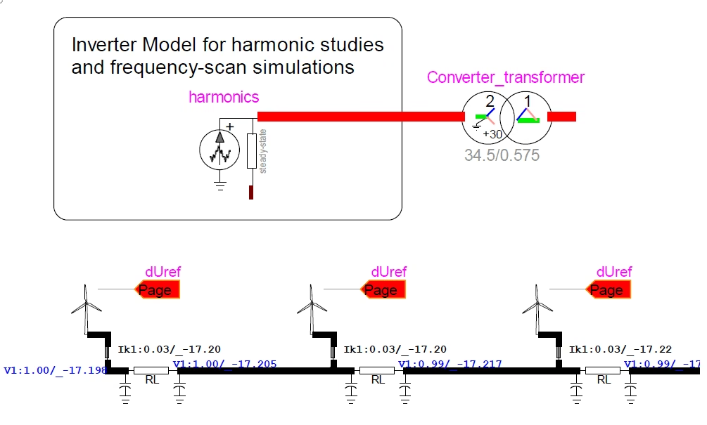
Top: an inverter model for harmonic and frequency-scan studies, drawn as a harmonic current source with a steady-state block feeding through a converter transformer (34.5/0.575 kV, delta-wye, +30 degrees). Bottom: a collector feeder with three wind-turbine inverters, each with a dUref page reference, showing per-bus current and voltage phasors such as V1 = 1.00 pu at -17.20 degrees and Ik1 = 0.03 pu at -17.20 degrees, with the angles changing slightly from bus to bus along the feeder. — Figure 1 — The harmonic-study model: (top) the inverter as a harmonic current source injecting its measured harmonic spectrum through the converter transformer, in place of an explicit PWM-switching model; and (bottom) a collector feeder of several such inverters, each carrying its per-bus current and voltage phasors, whose small angle differences along the feeder shape how the harmonic currents sum.

Section 3

Why not model the switching

Modelling every IGBT in switching detail would force a very small timestep and an expensive simulation, and it would still need accurate OEM switching detail to be trustworthy — all to answer a question that is really about the injected spectrum, not the internal pulse pattern. Using the measured harmonic spectrum is therefore both more practical and often more reliable: the manufacturer’s emission data already captures what the real inverter injects, validated by test, without reconstructing it from first principles. It is the same realism-versus-cost trade-off that runs through all renewable modelling.

Section 4

The harmonic data table

The model mask carries a harmonic data table. For each harmonic it needs the harmonic order (and hence its frequency), the current magnitude as a percentage of the fundamental, and the phase angle together with the reference convention it is measured against. The phase-angle convention is not an optional extra — without it the magnitudes alone cannot be summed correctly. A representative spectrum looks like this:

Table 1 — A representative inverter harmonic-current spectrum (illustrative manufacturer data).
Harmonic \(h\)	Current magnitude (% of \(I_1\))	Angle Offset (deg)
1 (fundamental)	100	from load flow (e.g. −17.2)
2	0.41	0
3	0.17	0
5	0.72	0
7	0.20	0
11	0.071	0
13	0.17	0
15	0.092	0
17	0.087	0
19	0.064	0

So a 5th-harmonic entry of 0.72% means \(I_5=0.0072\,I_1\). Each harmonic current is built from the table and anchored to the inverter’s actual fundamental phase:

\[ \underline{I}_h = \frac{m_h}{100}\,I_1 \,\angle\, \big(\theta_1 + \Delta\theta_h\big) \]

\(\underline{I}_h\): harmonic-\(h\) current phasor
\(m_h\): magnitude from the table (% of the fundamental)
\(I_1,\theta_1\): fundamental current magnitude and angle (from the load flow)
\(\Delta\theta_h\): harmonic angle offset from the table

The first line’s (fundamental) current angle is added to the angle of every other harmonic, so the whole spectrum rotates with the fundamental. The harmonic angle is a difference relative to the fundamental, not an absolute value set in isolation.

Section 5

The frequency-dependent network

Knowing the injected spectrum is only half the problem; the network response is the other half, and it is the heart of harmonic analysis. Transmission lines, cables and RLC elements are frequency dependent — a network does not react the same way at 50 or 60 Hz as at 250, 500 or 1000 Hz. The same injected harmonic current can therefore produce very different harmonic voltages depending on the network impedance at that frequency. Renewable parks in particular have long medium-voltage cable networks whose distributed capacitance, together with transformer leakage reactance and any filter components, sets up the resonant frequencies that matter. Every cable, transformer, capacitor, reactor and filter contributes a frequency-dependent impedance, and the harmonic voltage at any bus is that impedance times the injected current:

\[ \underline{V}_h = \underline{Z}(h\omega_1)\,\underline{I}_h \]

\(\underline{V}_h\): harmonic-\(h\) voltage at the bus
\(\underline{Z}(h\omega_1)\): network impedance at the harmonic frequency (frequency dependent)
\(\underline{I}_h\): injected harmonic-\(h\) current

The resonance is a property of the network, not of the source: it arises when the collector-system inductance, capacitance and damping combine to give a high impedance at or near a harmonic frequency. Near such a parallel resonance the impedance \(\underline{Z}(h\omega_1)\) is large, so even a modest harmonic current produces a large harmonic voltage — the amplification harmonic studies exist to find. So the inverter spectrum alone is not enough; you must know the network frequency response too.

Section 6

Why model the park in detail

It is recommended to model the park in detail for harmonics. Each feeder contains cable sections, shunt capacitances, RL or RLC elements, transformer branches and a particular collection-system topology, and each of those has its own frequency response. Aggregate the park too much and you can lose local filtering effects, local amplification, phase shifts along the feeder, and resonance between branches: over-aggregation can hide local resonances, feeder-level amplification and cancellation between inverter groups. The difference may not be huge in every case, but it is real — so when harmonic accuracy matters, detailed modelling is preferred over a crude single-machine equivalent.

Section 7

The key challenge: the harmonic current angle

Here is the part that catches people out. With many inverters along a feeder, each injecting a harmonic current, the total harmonic current at the substation is not the arithmetic sum of the magnitudes. It is a phasor sum:

\[ \underline{I}_h^{\,\mathrm{bus}} = \sum_{k} \underline{I}_{h,k} = \sum_{k} |I_{h,k}| \,\angle\, \theta_{h,k} \]

\(\underline{I}_h^{\,\mathrm{bus}}\): total harmonic-\(h\) current at the collection point
\(\underline{I}_{h,k}\): harmonic-\(h\) current contributed by inverter \(k\)
\(\theta_{h,k}\): its phase angle

If two harmonic currents are aligned they add strongly; if misaligned they partly cancel. If the angles are ignored and the magnitudes are simply added, the study can significantly over- or under-estimate the harmonic current and the resulting voltage distortion. So the total distortion at a collection point depends on the harmonic magnitude, the harmonic angle, the network phase shifts and the loading — which is why harmonic studies can be surprisingly sensitive. Such a feeder of inverters, each with its own per-bus current and voltage phasors, is shown at the bottom of Figure 1.

Section 8

Anchoring the angles from a load flow

The load flow establishes the fundamental operating point, and the harmonic current components are then referenced to that fundamental phasor so each inverter injects its harmonics with the correct relative angle. Because the angles matter, they cannot be assigned arbitrarily — they must be tied to the real operating point. So the procedure is to run a load flow first, then the harmonic or frequency scan. The load flow gives each inverter’s operating-point voltage magnitude and angle and its fundamental current magnitude and angle; even at the fundamental, each inverter’s current already has a particular phase, because buses have different voltage angles, feeder currents differ, and shunt capacitances create reactive paths. The harmonic injections are then referenced to those fundamental phasors, so the spectrum is anchored to where each inverter actually sits. The harmonic study is therefore not independent of the load flow — it is built on top of the load-flow solution, with all harmonics rotating consistently with the fundamental.

Section 9

Slight angle differences along the feeder

Look along a feeder and the current angles at different points differ only slightly — but those small differences can still matter, because the summation is a phasor effect. Even a modest angular mismatch changes the total current magnitude, the degree of cancellation or amplification, and the local voltage distortion, especially when many inverters contribute together. The practical lesson is that you should not assume all the sources are perfectly in phase unless that assumption is justified; the load-flow-anchored angles are what keep the picture honest.

When measured harmonic angles are not available, a common fallback is to assume the harmonic currents are aligned; that gives a conservative, worst-case sum, but it may be unrealistic. A good study states explicitly which angle assumption it uses — measured, manufacturer-supplied, random or statistical, or worst-case aligned — because the result depends on it.

Section 10

The converter transformer

The inverter harmonic source connects through its converter transformer, and that transformer is part of the harmonic picture too. Its leakage reactance, winding impedance and phase shift are frequency dependent, and it can interact with the cable capacitances to create local resonance. So even before a harmonic current reaches the main collection system, it has already been shaped by the local transformer and feeder connection — another reason a detailed park model, rather than an aggregated one, is worth building when harmonics are the focus.

The transformer is not the only local shaping element. On the grid-side converter it is common to add a small shunt ac harmonic filter next to the choke, arranged as two band-pass branches tuned to the switching-frequency harmonics, so the sharpest part of the converter emission is trapped locally before it ever reaches the collector network. The two branches sit at the first switching-related order and its second, and are made deliberately sharp with a high quality factor:

\[ n_1 = \frac{f_{\mathrm{PWM}}}{f_s}, \qquad n_2 = 2\,n_1, \qquad Q = 1000 \]

\(n_1\): tuning order of the first band-pass branch, at the switching-frequency harmonic
\(n_2\): tuning order of the second branch, at twice \(n_1\)
\(f_{\mathrm{PWM}}\): converter switching (PWM carrier) frequency
\(f_s\): fundamental (system) frequency
\(Q\): branch quality factor, set high (here 1000) for a narrow, sharply tuned notch

The branch reactances follow from the filter’s reactive-power rating and the rated low-voltage terminal voltage, in the usual \(Q_{\mathrm{filter}}=V_{\mathrm{LV}}^2/X\) way. Because these tuned branches shape the emission at source, a detailed harmonic model should represent them explicitly rather than folding them into an aggregate — they change what the converter actually injects into the feeder.

Section 11

Frequency scan versus harmonic analysis

Harmonic work groups two related but distinct tasks, and it is worth keeping them apart:

Table 2 — Frequency scan and harmonic analysis, and how they complement each other.
Study	What It Does	What It Tells You
Frequency scan	Sweeps frequency and computes the network impedance \(Z(f)\)	Where the network resonates, amplifies or is weakly damped
Harmonic analysis	Injects the measured harmonic spectrum at each inverter	The actual harmonic voltages, currents and distortion that result

The two support each other: the frequency scan tells you where the network is sensitive, and the harmonic analysis tells you what distortion actually appears when the sources inject their spectrum. The headline outcome is the distortion at each bus — most often the voltage total harmonic distortion:

\[ \mathrm{THD}_V = \frac{\sqrt{\displaystyle\sum_{h\ge 2} V_h^{2}}}{V_1} \]

\(\mathrm{THD}_V\): voltage total harmonic distortion at the bus
\(V_h\): magnitude of the harmonic-\(h\) voltage
\(V_1\): fundamental voltage magnitude

THD is a single summary index of distortion relative to the fundamental; it is useful, but the individual harmonic magnitudes are still needed, because limits and resonance risks are often frequency-specific. The THD and the individual harmonic levels are compared against the applicable limits — assessment frameworks such as IEC 61400-21 and IEEE 519 provide indices and limits that depend on the project jurisdiction and connection requirements rather than a single universal value — and, where they are exceeded, passive or active harmonic filters may be specified.

Section 12

The study workflow

Put together, the harmonic lab runs as a practical sequence:

Define the operating point for the study — the dispatch, control mode and grid-voltage condition the emission data should match.
Build the collector-grid model in detail, with frequency-dependent cables, transformers and RLC elements.
Run a load flow to obtain each inverter’s fundamental current magnitude and angle and the bus voltage angles.
Assign the harmonic spectra and phase angles (measured or manufacturer data) to each inverter, referenced to its load-flow operating point so the spectrum is correctly aligned.
Run the frequency scan to map the network impedance and locate resonances.
Inject the harmonics and run the harmonic analysis.
Check the bus voltages, branch currents, THD and individual harmonic levels against the applicable limits, and note any resonant issues.

In one sentence

Harmonic studies of renewable parks inject manufacturer-provided harmonic spectra into a detailed, frequency-dependent network, with source magnitudes and angles aligned from the load-flow operating point.

Section 13

Key points

Inject a measured spectrum, anchor the angles, trust the network response

For harmonic and frequency-scan studies the inverter is a harmonic current source injecting a measured, manufacturer-provided spectrum — not an explicit switching model.
The harmonic angles matter, because along a feeder the currents add as a phasor sum: aligned ones reinforce, misaligned ones cancel, and a load flow is run first to anchor them to the fundamental.
The collector network is frequency-dependent, so the harmonic voltage is \(\underline{V}_h=\underline{Z}(h\omega_1)\,\underline{I}_h\) and depends on the impedance at each frequency.
Resonance can amplify distortion: it is a network property — cable capacitance, transformer reactance and damping — so a detailed park model is preferred over a crude equivalent.
A frequency scan identifies the sensitive frequencies, while a harmonic analysis quantifies the harmonic voltages, currents and THD at each bus against the applicable limits.

For the park itself and the resonance / weak-grid side, see the PV park modelling and SSCI / frequency-scan guides.

References

EMTP® Documentation and Application Notes. Powersys / EMTP®.

Built on EMTP® · Expert spotlight

Henry Gras

Chief Operating Officer, PGSTech · Montréal, Canada

Henry Gras delivers the EMTP® University course “EMT Simulation and Analysis of Large-Scale Power Systems with Renewables” and works daily with the tool this article is written around.

Henry is based in Montréal, where he is Chief Operating Officer of PGSTech, the company responsible for EMTP® engineering services, commercialisation and continuing software development. He holds a master’s degree from Polytechnique Montréal, where he worked on electrical-machine research, and previously completed an engineering degree at École Centrale de Lyon in France.

Readers who want a structured programme on EMT simulation of large-scale power systems with renewables will find his EMTP® University course an excellent next step.

Henry’s technical expertise covers electromagnetic transient simulation, renewable-energy integration, power-system modelling, electrical machines, protection and specialist transient studies including TRV, transformer energisation, ferroresonance, insulation coordination and power quality.

Part 25 Reading now

Harmonic and Frequency-Scan Studies of Renewable Parks

Harmonic current sources, injection angles and the network frequency response of a renewable park.

Series progress 25 of 30

Part 26

Time-Domain Impedance Scanning for SSCI

Time-domain impedance scanning that combines the grid and turbine impedance for SSCI screening.