Renewable Modelling · PV Park

PV Park Modelling in EMTP®: Aggregated Architecture and Study-Dependent Representation

A solar park, like a wind park, is one top-level model in EMTP® that quietly changes what it is depending on the study. For a load flow it is a simple PQ injection; for a time-domain EMT run it is a detailed aggregated converter and control model; for a harmonic study it is an ideal harmonic source. Structurally it is the PV analogue of the DFIG wind park — only the energy source differs, with irradiance and a dc stage in place of the wind and the machine. This focused guide covers what is specific to PV and cross-references the wind-park and initialisation guides for the mechanics they share.

Reading time ≈ 16 min · PV park architecture & study modes

A photovoltaic park and a wind park are, to EMTP®, almost the same object. Both are modelled as a single aggregated plant whose internal representation changes with the study; both reduce to a PQ injection for load flow, lean on an ideal-source trick to initialise, and aggregate their collector network and unit transformers. The honest way to present a PV park is therefore to point at what it shares with the wind park — the layered architecture and aggregation, the load-flow PQ branch and ideal-source initialisation, and the reasons initialisation matters at all — and then spend the time on what is genuinely different: the source. This focused guide does exactly that.

Abbreviations used on this page

PVPhotovoltaic (solar)

EMTElectromagnetic transient (time domain)

EMTP®Electromagnetic Transients Program

LFLoad flow

PQConstant active / reactive power injection

PPCPlant (park) controller

PCCPoint of common coupling (grid connection)

PLLPhase-locked loop (converter synchronisation)

dcDirect-current side of the inverter

acAlternating-current (grid) side of the inverter

MPPTMaximum power point tracking (dc-side operating point)

\(G\)Solar irradiance (W/m²)

STCStandard test conditions (\(1000\,\text{W/m}^2\), 25 °C cell)

PWMPulse-width modulation (inverter switching)

Key idea

A PV park in EMTP® is one aggregated top-level plant whose internal representation switches with the study: a PQ / load-flow branch, a detailed time-domain converter branch, and a harmonic-source branch.
The PV-specific part is the source: an irradiance-driven PV array and dc side, with active power bounded by irradiance, temperature, set-point and the inverter rating. The grid-facing behaviour is governed by the inverter’s capability and current limits, the plant controller and the chosen study representation.
Load flow uses only the PQ branch (its breaker open, the detailed converter disconnected); at the start of the EMT run the same device becomes an ideal voltage source that both lets the plant initialise behind a stiff terminal and shields the grid by holding the load-flow power — then it is released.
The model is aggregated (equivalent collector grid, aggregated converter transformer, optional capacitor bank and grounding) and supervised by the PPC at the PCC. Its named internal structure drives the automation, so the device names must not be changed.

Key terms used on this page

01PV park

An aggregated solar plant: PV panels, inverters, collector network and transformers, modelled as one device.

02PQ-initialisation branch

The simplified branch used during load flow, where the park is a specified active/reactive injection.

03Ideal voltage source

A temporary stiff terminal used at EMT start so the plant can initialise without disturbing the grid.

04Plant controller (PPC)

Supervisory controller that meets the voltage/reactive/power-factor target at the PCC.

05Aggregated model

Many identical units represented by one equivalent, with ratings and impedances scaled accordingly.

06Equivalent collector grid

A reduced circuit reproducing the impedance and charging of the plant’s medium-voltage cable network.

07Converter transformer

The inverter-unit step-up transformer (commonly 1–2 MVA per unit), aggregated to one equivalent.

08Harmonic-source branch

The representation swapped in for harmonic or frequency-scan studies in place of the switching model.

09Irradiance

Incident solar power per unit area; it sets the available dc power, much as wind speed does for a turbine.

10Study-dependent representation

One top-level device whose active internal branch is chosen by the study: load flow, EMT or harmonic.

Section 1

Same architecture, a different source

Structurally, a PV park is generic converter-plant scaffolding wrapped around a solar source. The grid side — the aggregated converter transformer, the equivalent collector grid, optional shunt compensation, the park transformer and a supervisory plant controller — is the structure already covered for the DFIG wind park, and it behaves the same way here.

The rest of this page therefore concentrates on that one PV-specific part — how a solar plant produces its power — and then follows it into the shared load-flow, initialisation and study-mode machinery.

The through-line

The load-flow PQ branch, the ideal-source initialisation and the aggregation are shared with any converter plant; what is PV-specific is the source — the PV array, its irradiance and temperature response, the dc side, the MPPT and the inverter limits.

Section 2

The PV source: irradiance and the dc side

A wind turbine’s power comes from a rotating mechanical drive train; a PV plant’s comes from an irradiance-driven dc source. The PV array provides dc power whose maximum available value depends on the irradiance and the module temperature; maximum power point tracking (MPPT) sets the dc-side operating point to extract that available power — up to the point where the inverter’s own ac rating clips it — though during a grid-code event or curtailment the plant may deliberately run below the maximum. On the dc-side representation — the array and dc link, which many inverter models capture without an explicit separate dc–dc converter — the inverter then exports the commanded active power to the ac network, subject to the available dc power, the inverter rating and the plant-level limits. Broadly, the available power scales with irradiance up to the inverter rating:

\[ P \approx \frac{G}{G_{\text{STC}}}\,P_{\text{rated}}\ \ (\le P_{\text{rated}}), \qquad \underline{S}_{\text{PCC}} = P + jQ \]

\(P\): active power the plant delivers (a high-level approximation only)
\(G\): incident solar irradiance
\(G_{\text{STC}}\): reference irradiance at standard test conditions, STC (\(1000\,\text{W/m}^2\))
\(P_{\text{rated}}\): the relevant plant / inverter active-power limit used by the model — the inverter ac rating, the plant export limit and the array dc rating are not always the same
\(\underline{S}_{\text{PCC}}\): complex power at the point of common coupling (PCC); sign convention here: positive \(P\) and \(Q\) are injection from the plant into the grid, unless the EMTP® / project convention is the opposite
\(j\): imaginary unit, \(j=\sqrt{-1}\)
\(Q\): reactive power, set by the control mode (fixed-\(Q\), power-factor or voltage)

This is a simplified explanatory relationship, not a full PV performance model: the actual output also depends on the module temperature, the MPPT operation, inverter clipping, any curtailment, losses and the plant set-point. What it captures is the essential PV difference — \(P\) is driven by irradiance rather than wind, with no shaft or machine — while reactive power is set as before, by the plant controller within the inverter’s capability.

For load flow this is all the network needs: a controlled \(P\) from the sun and a controlled \(Q\) from the plant controller. The detailed converter that produces them is only brought to life for a time-domain study.

A modelling caveat: MPPT is not dynamic here

In this aggregated generic model the MPPT algorithm itself is not simulated. The active-power reference is fixed at initialisation from the chosen operating point — the maximum available power in MPPT mode, or a specified value in power-control mode — so changing the irradiance part-way through a run does not, on its own, move the power reference. That is acceptable for the short time frame of an EMT study, where a fault or switching event (not a passing cloud) is the disturbance of interest; it simply means this model is not the tool for slow irradiance-ramp or MPPT-tracking studies.

Section 3

Reading the model, left to right

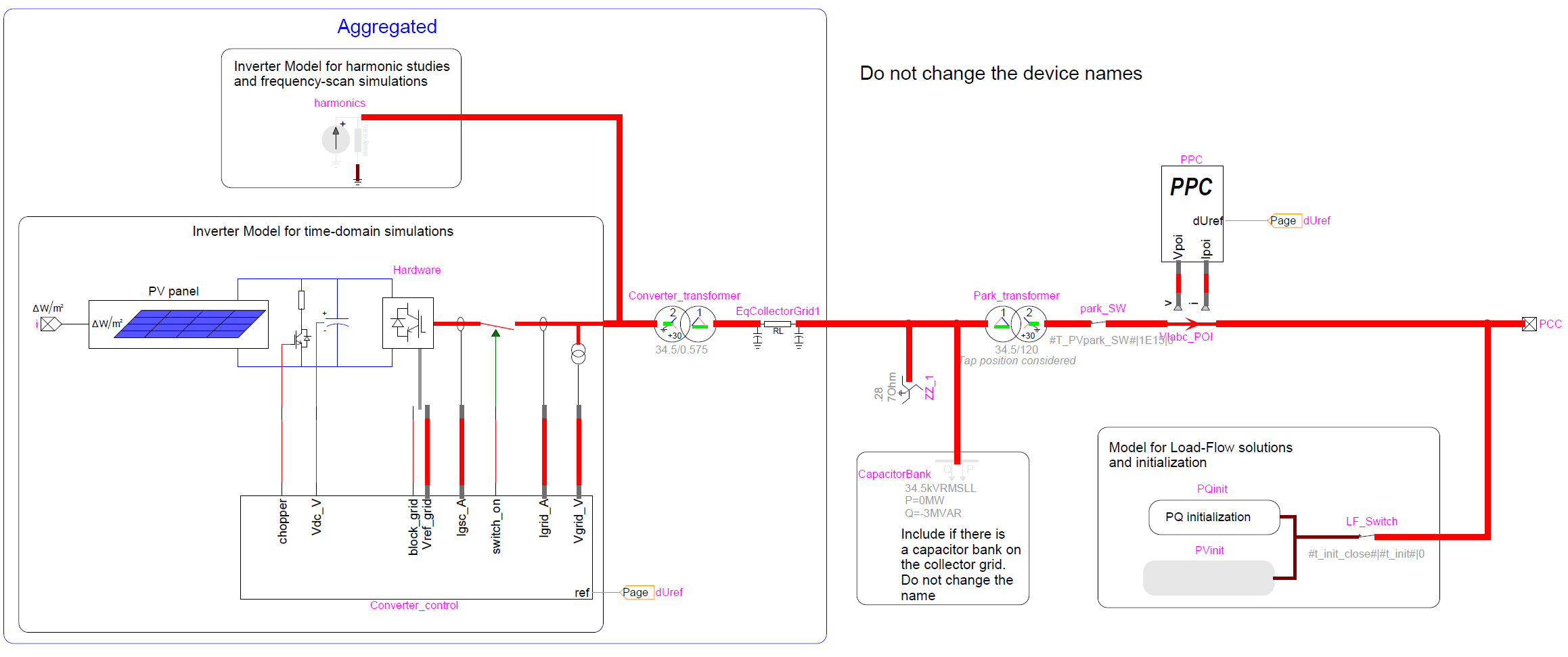
The PV-park schematic reads as a layered plant from the source out to the grid:

PV source — irradiance drives the PV panel and sets the available dc power.
Detailed converter block — the inverter hardware and converter controls turn dc into ac.
Aggregated converter transformer — the inverter-unit step-up, combined into one equivalent.
Equivalent collector grid — the internal medium-voltage network, in aggregated form.
Plant-level components — grounding representation and an optional capacitor bank, where present.
Park transformer — steps the collector voltage up to the connection level; its tap position is treated as a fixed parameter, with on-load tap-changer (OLTC) motion not modelled dynamically in this representation.
Plant controller (PPC) — supervises the voltage/reactive/power-factor target at the PCC.
Load-flow / initialisation branch — solves the operating point first, then supports a smooth transition into EMT.
Harmonic branch — for harmonic or frequency-scan work, swapped in for the time-domain converter path.

Aggregated PV-park model in EMTP: the irradiance-driven PV source and detailed inverter block, the harmonic-source block, the aggregated converter and park transformers, the equivalent collector grid, the optional capacitor bank, the plant controller (PPC), the PCC, and the load-flow / initialisation branch. — Figure 1 — The aggregated PV-park model: an irradiance-driven PV source and detailed inverter (used for time-domain EMT), a separate harmonic-source block (used for harmonic / frequency-scan studies), the aggregated converter transformer, equivalent collector grid, optional capacitor bank, park transformer and plant controller (PPC), and the load-flow / initialisation branch that solves the operating point and supports the transition into EMT.

Section 4

The plant controller (PPC)

The block labelled PPC (the PV plant controller) is the plant-level supervisory controller. It measures what the plant is doing at the PCC, compares that against the target — a reactive-power, voltage or power-factor set-point — and trims the reference sent to the aggregated converter so the whole plant meets it, deliberately slower than the converter’s inner loops. But two limits decide whether the reference can actually be met. The PPC only creates the reactive-power or voltage-support reference; whether the inverter can deliver it depends on the inverter’s capability curve and current limit. PV inverters have an apparent-power (current) limit, so at high active-power output the available reactive capability is reduced unless the inverter is oversized or active power is curtailed — which matters directly for voltage-control and fault-ride-through studies.

Section 5

Aggregation: one equivalent plant

A real PV plant has many identical inverter-and-transformer units on an extensive collector network. Past the collector side, EMTP® stops tracking each physical unit and represents the plant by equivalent aggregated blocks. The scaling is book-keeping once the number of units \(N\) and their rating are known: the total rating scales with \(N\), and because the transformer data are usually held in per unit on their own base, the equivalent is assembled on the appropriate per-unit / MVA base rather than by manipulating raw ohms.

The aggregated converter transformer combines the many inverter-unit transformers (commonly 1–2 MVA each) into one equivalent on the appropriate base.
The equivalent collector grid reproduces the series impedance, shunt charging, voltage drop and losses of the internal cable network. For load-flow studies this equivalent mainly needs to capture the voltage drop and the reactive charging; for harmonic or frequency-scan studies the distributed nature of the cable network can matter, and a more detailed representation may be needed so the charging and resonances land correctly.
Plant-level passive components — a grounding representation and an optional capacitor bank — are included where they exist in the real project. A capacitor bank affects voltage, reactive power and harmonic resonance; the grounding and transformer connections affect zero-sequence behaviour and unbalanced-fault studies — so each matters most in the study it touches.

This single aggregation assumes the inverter blocks are similar enough and see similar grid conditions. Where that does not hold — feeders that differ materially, or cases where cable charging, voltage drop or a collector-grid resonance matters — the plant is split into several aggregated blocks instead of one. Either way it is a plant model, not just a converter model: it carries the equivalent of everything from the inverter terminals out to the PCC.

Section 6

Load flow: only the PQ branch

During a load-flow solve, only the load-flow branch of the PV park is active and the rest is set aside: the detailed converter is not running, the controller is not solved as a dynamic system, and the PV array is not simulated as a switching device. What remains is a controlled PQ injection — a specified active power with a specified or controlled reactive power. This is an algebraic steady-state representation of what the plant delivers at the PCC, not a physical model of the source: the load flow needs the injected \(P\) and \(Q\), not the switching detail behind them.

The branch is switched in for the load-flow solve and out for the detailed run by the model’s own load-flow switches, so the PQ device and the detailed plant are never active together. The full switch logic — which breaker is open in which mode, and why — is the same arrangement documented on the dedicated load-flow and initialisation page; here it is enough that the steady-state injection reaches the network cleanly, without wrong coupling to internals that take no part in the steady-state solution. Only the origin of \(P\) — sunlight rather than wind — differs.

Section 7

Initialisation: the ideal source’s two jobs

At the start of the time-domain run the detailed PV model must be brought into operation, but its controls and converter states are not yet correctly set. So the load-flow device temporarily becomes an ideal voltage source that supports the plant while it settles. This is temporary numerical support, not part of the study: what the plant does during the initialisation window is a settling transient, not a result to be measured. It does two jobs at once.

It helps the plant initialise. From the PV park’s side the source is a very strong grid — a fixed voltage magnitude and angle — giving the PLL, the inner current loops, the outer loops, the dc-side variables, the measurement filters and the plant-controller signals a quiet, stiff environment in which to settle quickly.
It shields the grid. From the network’s side the source holds the power exchange at the load-flow values, so the external system keeps seeing the correct \(P\) and \(Q\) and there is no start-up ramp that could create a stability problem — important when many plants share a weak grid and would otherwise perturb one another.

How long this takes is model-dependent: it is set by the slowest states that must reach equilibrium — the PLL, the inner current loops, the dc-link voltage, the outer and plant-level (PPC) loops and any limiters — so a plant with slow outer control needs a longer window than one with fast control only. Once those states have settled, the source is removed and the detailed plant takes over with only a small disturbance. After release it is worth checking in the time domain that \(P\), \(Q\) and the terminal voltage hold at the load-flow values and do not drift — the practical confirmation that the hand-over was clean. The mechanism and timing match the converter-plant initialisation; a synchronous machine, by contrast, can be initialised directly without it.

Section 8

One device, three forms

The single most useful property of the model is that one top-level device exposes a different internal representation for each kind of study. These are not three separate physical objects: they are alternative representations of the same plant, only one of which is active at a time, so a user keeps one organised plant with its data in one place instead of maintaining several drifting versions.

Table 1 — One PV-park device, three internal representations selected by the study.
Study	Active Internal Branch	Detailed Converter?
Load flow (steady state)	PQ-initialisation branch only	No — detailed converter disconnected
Time-domain EMT	Time-domain aggregated converter model — detailed switching or average-value — with its control and PV source	Yes (switching or average-value)
Harmonic / frequency scan	Ideal harmonic-source representation	No — replaced by a harmonic source

The harmonic branch carries an important caution. The harmonic source is only as good as the data behind it — its injected magnitude and phase spectrum, and the converter impedance it presents, all have to match the study being run. And a model built for grid-code or fault-response studies is not automatically suitable for harmonic work: getting harmonics right depends on the converter’s impedance, the control-loop response at the frequencies of interest, the filters, the transformer and the cable capacitance — not on how faithfully it reproduces a fault. So always ask what a converter model was built for before trusting its harmonic output; this is the same point made in the study-workflow guide.

Section 9

Why “do not change the device names”

The model comes with a blunt instruction: do not change the device names. It is not cosmetic. Models at this level rely on named internal structure — internal scripting, named links, masked parameters, the automatic adaptation between study types, and initialisation logic tied to specific block names. Rename a device casually and you can break those internal references, the automation, the initialisation, or the switching between load-flow, time-domain and harmonic modes. The names are part of how the model works, so they are left alone.

Practical rule

Treat the supplied block names as fixed. Configure the plant through its parameters and options, not by renaming its internal devices.

Section 10

Key points

One plant, a study-chosen representation, a PV source

EMTP® models a PV park as one aggregated plant whose internal representation is chosen by the study — a PQ branch for load flow, a time-domain converter model (switching or average-value) for EMT, and a harmonic source for frequency-scan work. What is genuinely PV is the source: an irradiance- and temperature-driven array and dc side, with active power bounded by irradiance, set-point and the inverter rating, and reactive capability limited by the inverter’s current at high output. The grid-facing scaffolding — aggregated collector grid and converter transformers, a plant controller that meets the target at the PCC, the load-flow PQ branch and the ideal-source initialisation — is shared with other converter plants, and the named internal structure must be left intact for the automation to work. For the shared mechanics, see the wind-park architecture, the load-flow and initialisation guide, and the synchronous-machine initialisation and study workflow.

References

EMTP® Documentation and Application Notes. Powersys / EMTP®.

Built on EMTP® · Expert spotlight

Henry Gras

Chief Operating Officer, PGSTech · Montréal, Canada

Henry Gras delivers the EMTP® University course “EMT Simulation and Analysis of Large-Scale Power Systems with Renewables” and works daily with the tool this article is written around.

Henry is based in Montréal, where he is Chief Operating Officer of PGSTech, the company responsible for EMTP® engineering services, commercialisation and continuing software development. He holds a master’s degree from Polytechnique Montréal, where he worked on electrical-machine research, and previously completed an engineering degree at École Centrale de Lyon in France.

Readers who want a structured programme on EMT simulation of large-scale power systems with renewables will find his EMTP® University course an excellent next step.

Henry’s technical expertise covers electromagnetic transient simulation, renewable-energy integration, power-system modelling, electrical machines, protection and specialist transient studies including TRV, transformer energisation, ferroresonance, insulation coordination and power quality.

Part 4 Reading now

PV Park Modelling

Aggregated PV-park architecture and how the representation depends on the study you are running.

Series progress 4 of 30

Part 5

Plant-Controller Reactive Power Control

Plant-level Q, V and power-factor modes and the secondary voltage control that coordinates the park.