Renewable Modelling · Phase-Locked Loop (PLL)

The Phase-Locked Loop in EMTP® Converter Models

SRF-PLL dq alignment, lock dynamics and weak-grid sensitivity

The phase-locked loop (PLL) estimates the grid voltage’s angle and frequency, and that angle drives every dq transformation in the converter controller. If the angle is wrong — even slightly — the voltages, currents and powers the controller computes in dq are wrong with it. The synchronous-reference-frame (SRF) PLL used in EMTP® renewable models finds the alignment by forcing the q-axis voltage toward zero. It is a nonlinear dynamic system with its own bandwidth, and one of the main control paths through which a converter interacts with a weak grid, unbalance and impedance-based stability.

Reading time ≈ 20 min · SRF-PLL, q-axis lock & weak-grid dynamics

The phase-locked loop answers one question: what is the present angle and frequency of the grid voltage? It sounds modest, but the answer underwrites the whole converter controller. Vector control works in dq coordinates, and dq coordinates only mean anything if the rotating frame is aligned with the grid-voltage vector. The PLL is the block that finds and tracks that alignment, then hands the angle to every transform, current loop, power calculation and sequence extractor downstream. It is also, for the same reason, one of the main reasons converter behaviour changes in weak grids, under unbalance and in impedance-based stability work — a slightly wrong angle quietly corrupts everything built on top of it.
Abbreviations used on this page
PLLPhase-locked loop
SRF-PLLSynchronous-reference-frame PLL
EPLLEnhanced PLL
DSRFDouble synchronous reference frame
dqDirect–quadrature rotating frame
\(\alpha\beta\)Stationary (Clarke) frame
PIProportional–integral controller
LPFLow-pass filter
\(v_q\)q-axis grid voltage
\(\omega,\theta\)Angular frequency, phase angle
SSCISub-synchronous control interaction
EMTP®Electromagnetic Transients Program
Key idea
  1. The PLL estimates the grid voltage’s angle and frequency and supplies the rotating angle that every dq transform, current loop, power calculation and sequence extractor depends on. Without it the converter does not know where the grid-voltage vector is.
  2. The synchronous-reference-frame PLL aligns the d-axis with the voltage vector by driving the q-axis voltage to zero: transform \(v_{abc}\to v_{dq}\) with the estimated angle, low-pass filter and PI-regulate \(v_q\) toward zero to get the estimated frequency, integrate to get the angle, feed it back. At lock, \(v_q\approx 0\) and the frame rotates at grid frequency.
  3. The PLL is a nonlinear dynamic system with its own bandwidth and settling time. Its transient corrupts not just the angle but every dq voltage, current and power the controller computes — so PLL dynamics shape the whole converter response.
  4. That is why the PLL is central to weak-grid stability and SSCI, and why unbalance — negative sequence appearing as a twice-grid-frequency ripple in \(v_q\) — demands a DSRF or enhanced PLL. Tuning is a speed-versus-robustness trade-off.
Key terms used on this page
01Phase-locked loop
A feedback loop that estimates and tracks the grid-voltage angle and frequency.
02SRF-PLL
The synchronous-reference-frame PLL: transform to dq, drive the q-axis voltage to zero.
03dq frame
A frame rotating with the estimated angle, in which balanced AC quantities look constant.
04q-axis voltage
The component the SRF-PLL nulls; near lock it is a near-linear measure of the angle error.
05Lock condition
Steady state where \(v_q\approx 0\), the d-axis is aligned, and the frequency estimate is correct.
06PLL bandwidth
How fast the loop tracks angle and frequency changes; sets settling time and disturbance sensitivity.
07Frequency estimate
The PI output; integrating it produces the phase angle.
08Phase angle
The rotating angle fed to every dq transformation in the controller.
09Negative sequence
The reverse-rotating component under unbalance; appears at twice fundamental frequency in dq.
10DSRF
Double synchronous reference frame: two counter-rotating frames that separate the sequences cleanly.
11EPLL
Enhanced PLL: an adaptive structure with better rejection of harmonics and distortion.
12SSCI
Sub-synchronous control interaction: a converter–grid instability the PLL strongly influences.

Section 1

What the PLL is for

The PLL must estimate two things: the frequency \(\omega\) (or \(f\)) and the phase angle \(\theta=\omega t\) of the grid voltage. These are needed because the converter controller is built in dq coordinates, and the dq frame only makes sense if it is aligned with the grid voltage. So the PLL provides the rotating angle used by the abc→dq transformation, the current control, the voltage control, the power calculation and — in more advanced controllers — the sequence extraction. It is the reference everything else is measured against.

One angle, used everywhere

The PLL is not a peripheral measurement. It produces the single rotating angle that defines the controller’s coordinate system — so its accuracy and its dynamics propagate into every dq quantity the converter acts on.

Section 2

Why dq needs an angle

The dq transformation came from synchronous-machine analysis, where a frame rotating with the rotor makes the machine inductances look constant instead of time-varying. For converters and renewables the dq frame is kept for two practical reasons. First, a balanced AC quantity becomes almost constant in steady state, so a simple PI regulator can drive it to a set-point with zero steady-state error. Second, active and reactive control separate cleanly along the d and q axes, which makes the current and power loops straightforward to design. But the dq frame is defined relative to a rotating angle, and that angle has to come from somewhere. The PLL is what supplies it — which is why it is not an optional extra but the thing that makes dq control possible at all.

Section 3

Forcing the q-axis voltage to zero

The synchronous-reference-frame PLL transforms the measured three-phase voltage into dq using a trial angle. If that angle is correct, the d-axis aligns with the voltage vector and the q-axis voltage is zero. That is the whole principle — the SRF-PLL drives \(v_q\) to zero. Projecting the voltage vector onto the estimated frame gives:

\[ v_d = \hat{V}\cos(\theta - \hat{\theta}), \qquad v_q = \hat{V}\sin(\theta - \hat{\theta}) \]
\(v_d,\ v_q\)
grid voltage resolved in the estimated dq frame
\(\hat{V}\)
peak phase-voltage magnitude
\(\theta\)
true grid-voltage angle
\(\hat{\theta}\)
angle estimated by the PLL

If the frame leads or lags the true angle, \(v_q\) is non-zero — positive one way, negative the other — so it is a signed error. For a small error, \(v_q\approx\hat{V}(\theta-\hat{\theta})\): the q-axis voltage is a near-linear measure of the angle error, and that is exactly the signal the PLL drives to zero.

The sign of \(v_q\) depends on the dq (Park) transform convention used, so EMTP®, PSCAD, PowerFactory and textbook conventions can differ; the PLL principle is unchanged, because the loop is tuned to drive \(v_q\) toward zero whichever sign applies.

Section 4

The synchronisation loop

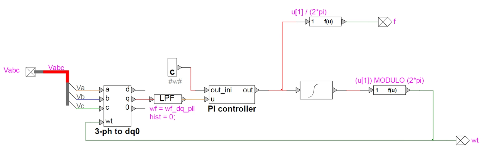
The loop runs in order. The measured voltage \(v_{abc}\) is transformed to dq using the present estimated angle. The q-axis voltage is low-pass filtered — measurements carry noise, harmonics and switching ripple, and a cleaner signal makes the regulator better behaved. A PI controller then drives the q-axis voltage toward zero; this is the angle-and-frequency regulation loop. The PI output is, in effect, a frequency, and integrating a frequency gives an angle — so an integrator turns it into the estimated angle, which is fed straight back into the dq transformation. The loop closes on itself.

\[ \hat{\omega} = \omega_n + \left(k_p + \frac{k_i}{s}\right) v_q, \qquad \hat{\theta} = \int \hat{\omega}\,dt \ \ (\mathrm{mod}\ 2\pi) \]
\(\hat{\omega}\)
estimated angular frequency (PLL output)
\(\omega_n\)
nominal feed-forward frequency (e.g. \(2\pi\cdot 50\) rad/s)
\(k_p,\ k_i\)
PI gains that set the loop bandwidth and damping
\(v_q\)
filtered q-axis voltage — the loop error
\(\hat{\theta}\)
estimated angle, wrapped to \([0,2\pi)\), fed back to the transform

The PI drives \(v_q\) to zero; its output is the frequency estimate; the integrator turns that into the angle. The nominal feed-forward \(\omega_n\) gives the loop a sensible starting point so it only has to correct the deviation from nominal.

Synchronous-reference-frame (dq-based) PLL block diagram in EMTP: the three-phase voltage Vabc enters a three-phase-to-dq0 transform driven by the estimated angle wt; the q-axis output passes through a low-pass filter and a PI controller; the PI output is integrated and taken modulo 2-pi to form the angle wt fed back to the transform, and scaled by 1/(2-pi) to give the frequency f.
Figure 1 — The synchronous-reference-frame PLL: the three-phase voltage is transformed to dq using the estimated angle, the q-axis voltage is filtered and driven to zero by the PI regulator, and the PI output is integrated to produce the angle (and frequency) fed back to the transform.

Section 5

Frequency and angle

One basic relationship sits at the heart of every PLL: frequency is the rate of change of angle. So if the PI gives a frequency estimate, the angle is obtained by integrating it.

\[ \omega = \frac{d\theta}{dt} \qquad\Longleftrightarrow\qquad \theta(t) = \theta_0 + \int_0^{t}\omega\,d\tau \]
\(\omega\)
angular frequency
\(\theta\)
phase angle
\(\theta_0\)
initial angle at \(t=0\)

Every PLL therefore contains a frequency estimator and an integrator for the angle, and produces two outputs: \(\omega\) and \(\theta\). The angle is the one the dq transformations need most directly.

Section 6

The lock condition

When the PLL is locked in steady state, four things are true together: the estimated angle rotates at the correct grid frequency; the q-axis voltage \(v_q\approx 0\); the d-axis is aligned with the grid-voltage vector; and the frequency estimate is correct — 50 Hz on the GB system, 60 Hz elsewhere. A locked PLL is simply the statement that the converter’s frame is synchronised with the grid.

Locked

\(v_q\approx 0\), the d-axis tracks the voltage vector, and \(\hat{\omega}\) equals the grid frequency. Everything the controller does in dq is then referenced to a frame that genuinely follows the grid.

Section 7

The PLL has dynamics

The PLL is not instantaneous. If the grid frequency changes or the angle jumps, the loop needs time to respond: a frequency step might settle over something like a tenth to a couple of tenths of a second, depending on the tuning. That means the PLL is itself a dynamic system with a bandwidth, a settling time, some overshoot or damping, and a sensitivity to disturbances. Because every converter control loop depends on the PLL angle, those PLL dynamics flow through into the entire converter response — the current loop cannot be faster than the angle it is referenced to is trustworthy.

Section 8

Why it is nonlinear

A PLL cannot be reduced to a single fixed transfer function. It is nonlinear for several reasons at once. The dq transformation depends on the estimated angle, and that angle is itself the quantity being estimated, so the feedback path multiplies signals by the sine and cosine of the estimate. The transformation is trigonometric. The angle wraps modulo \(2\pi\). And under a large disturbance the small-signal approximation no longer holds. A small-signal linearisation around the lock point is still useful — it is how the loop bandwidth and stability margins are designed — but the block itself is fundamentally nonlinear, which is why a proper EMT model of the PLL matters: a linearised stand-in can hide exactly the behaviour that causes trouble.

Section 9

Weak grids and SSCI

If the PLL angle is even slightly wrong, the converter’s idea of \(v_d\), \(v_q\), \(i_d\) and \(i_q\) is wrong with it. The converter may then inject the wrong current, miscalculate its reactive support, create dq cross-coupling, reduce damping, and interact badly with the grid impedance. So the PLL is not just a measurement block: it sits inside the closed loop and is one of the main control paths through which the converter interacts with the grid impedance. In a weak grid, where that impedance is large and the short-circuit ratio is low, a fast PLL is a classic contributor to trouble — the angle moves with the converter’s own current, and the resulting feedback can produce sub-synchronous control interaction and negative damping in impedance-based stability scans. The PLL is rarely the only factor, but it is frequently part of the mechanism when a renewable plant shows a weak-grid oscillation.

Section 10

Unbalance and the twice-frequency problem

A balanced grid voltage transforms to a constant (dc) quantity in the synchronous dq frame. Negative sequence does not: because it rotates opposite to the dq frame, it appears in dq as an oscillation at twice the fundamental — 100 Hz in a 50 Hz system, 120 Hz in a 60 Hz system. That double-frequency component lands directly in \(v_d\) and \(v_q\), contaminating the very q-axis voltage the PLL is trying to null:

\[ v_q^{\,\mathrm{meas}} \approx \underbrace{\hat{V}^{+}(\theta-\hat{\theta})}_{\text{angle error}} \;+\; \underbrace{\hat{V}^{-}\sin(2\omega_1 t + \varphi^{-})}_{\text{negative-sequence } 2\omega_1 \text{ ripple}} \]
\(\hat{V}^{+},\ \hat{V}^{-}\)
positive- and negative-sequence voltage magnitudes
\(\omega_1\)
fundamental angular frequency
\(\varphi^{-}\)
negative-sequence phase

The first term is the error the PLL should act on; the second is a \(2\omega_1\) ripple it cannot distinguish from it. A plain SRF-PLL therefore ripples at twice grid frequency under unbalance — which is why a double synchronous reference frame or an enhanced PLL is used when the grid can be unbalanced.

This is exactly the choice the detailed EMTP® wind-park converter model makes for its synchronising angle. Instead of locking a plain SRF-PLL to the terminal voltages — whose angle would carry the \(2\omega_1\) ripple above — it derives \(\theta\) from a double-synchronous-reference-frame PLL that splits the terminal voltages into their positive- and negative-sequence parts and locks only on the positive sequence. The d-axis then stays aligned with the fundamental voltage vector, and the angle handed to every dq transform stays clean even when the grid is unbalanced — the same reasoning behind negative-sequence control.

Section 11

Tuning the PLL

PLL tuning is always a trade-off between tracking speed and robustness:

  • A fast PLL — better tracking of phase and frequency changes, but a higher risk of interacting with the grid impedance and amplifying weak-grid oscillations.
  • A slow PLL — better filtering and robustness, but poorer tracking during faults and fast phase changes, so the current loop can act on stale angle information.
  • Correct tuning — balances synchronisation speed, damping, sequence filtering and grid strength, chosen with the short-circuit ratio in mind rather than in isolation.
Common PLL pitfalls
  • A fast PLL in a weak grid. High bandwidth where the short-circuit ratio is low couples the angle to the converter’s own current and can drive an unstable interaction.
  • A plain SRF-PLL under unbalance. The \(2\omega_1\) ripple feeds straight through into the current references; sequence separation (DSRF / EPLL) is needed.
  • Treating the PLL as an ideal angle source. In EMT, SSCI and impedance studies, ignoring the PLL dynamics removes exactly the mechanism that shapes the result.

Section 12

Other architectures: the enhanced PLL

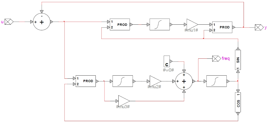
The dq-based SRF-PLL is the common baseline, but it is not the only structure — renewable models often also offer an enhanced PLL (EPLL) and sequence-separating variants. The teaching point is that “PLL” is not one universal fixed block: different architectures behave differently, and under distortion or unbalance the difference is large. More elaborate PLLs aim for better disturbance rejection, better harmonic filtering and cleaner performance when the grid is not ideal.

Table 1 — Common PLL architectures and where each fits.
ArchitecturePrincipleUnder UnbalanceTypical Use
SRF-PLLdq transform; drive \(v_q\to 0\)\(2\omega_1\) ripple in the estimate unless slowed or extra-filteredBalanced or mildly distorted grids — the baseline
EPLLAdaptive amplitude/phase estimator per phaseBetter rejection of harmonics and distortionPolluted, variable-frequency grids
DSRF-PLLTwo counter-rotating frames with cross-decouplingClean separation of \(+\) and \(-\) sequence; no \(2\omega_1\) rippleUnbalanced faults, sequence control
DSOGI-PLLSecond-order generalised integrators in \(\alpha\beta\)Good sequence separation and filtering togetherUnbalanced / distorted grids, FRT
Enhanced PLL (EPLL) block diagram in EMTP: the input u is compared with the estimated signal y to form an error; adaptive amplitude and phase-tracking loops (products, integrators and the mu gains) estimate the amplitude, phase angle and frequency, and a sine and cosine generator reconstructs y and the synchronisation signals.
Figure 2 — An enhanced PLL (EPLL). Different PLL architectures are not interchangeable: in EMT, SSCI and weak-grid work, the choice of structure can change the results noticeably.

Section 13

Key points

A nonlinear angle source the whole controller stands on

  1. Purpose. The PLL estimates the grid voltage’s angle and frequency and supplies the rotating angle used by every dq transform, current loop, power calculation and sequence extractor.

  2. SRF-PLL principle. It aligns the d-axis with the voltage vector by driving the q-axis voltage \(v_q\to 0\); at lock, \(v_q\approx 0\) and the frame rotates at grid frequency.

  3. Frequency to angle. The PI output is the estimated frequency; integrating it gives the angle that is fed back to the dq transform.

  4. Weak-grid sensitivity. As a nonlinear dynamic system inside the loop, the PLL is one of the main control paths for weak-grid and SSCI interaction; tuning trades speed against robustness.

  5. Unbalance. Negative sequence appears as a \(2\omega_1\) ripple in \(v_q\), so an unbalanced grid calls for a DSRF or enhanced PLL.

For the loops that use this angle, see the DFIG converter control, GSC current loop, DSC implementation and negative-sequence compensation guides.

References

References

  1. EMTP® Documentation and Application Notes. Powersys / EMTP®.
Built on EMTP® · Expert spotlight
Portrait of Henry Gras, Chief Operating Officer of PGSTech

Henry Gras

Chief Operating Officer, PGSTech · Montréal, Canada

Henry Gras delivers the EMTP® University course “EMT Simulation and Analysis of Large-Scale Power Systems with Renewables” and works daily with the tool this article is written around.

Henry is based in Montréal, where he is Chief Operating Officer of PGSTech, the company responsible for EMTP® engineering services, commercialisation and continuing software development. He holds a master’s degree from Polytechnique Montréal, where he worked on electrical-machine research, and previously completed an engineering degree at École Centrale de Lyon in France.

Readers who want a structured programme on EMT simulation of large-scale power systems with renewables will find his EMTP® University course an excellent next step.

Henry’s technical expertise covers electromagnetic transient simulation, renewable-energy integration, power-system modelling, electrical machines, protection and specialist transient studies including TRV, transformer energisation, ferroresonance, insulation coordination and power quality.

Thirty-Part Technical Series

EMTP® Renewable Energy Modelling

A thirty-part guide to modelling wind, PV and full-converter plant in EMTP® — sources and turbines, converter and plant control, sequence control under faults, protection, and weak-grid and SSCI stability.

Part 16 Reading now

The Phase-Locked Loop in Converter Models

SRF-PLL dq alignment, lock dynamics, and why the PLL becomes sensitive in a weak grid.

Series progress 16 of 30