Renewable Modelling · Initialisation & Flat Start

EMT Initialisation and Flat Start in EMTP®

Load-flow initialisation and block-by-block controller states

A reliable EMT simulation starts from a consistent steady-state operating point. Load-flow initialisation maps bus voltages, currents, converter states and controller memories into the EMT model so the first time step begins at equilibrium. Start instead from inconsistent or zero states and the model self-adjusts with artificial transients, long settling and, in a weak grid, false instability that looks real but is just bad initialisation. A clean flat start requires mapping the load-flow solution onto every EMT state — inductor currents, capacitor voltages, the PLL angle, and every controller block — hidden work that falls on the model developer, who initialises each block backward from its known steady-state output. What follows sets out why it matters, what gets initialised, and the block-by-block procedure, using the EXST1 exciter as the classic example.

Reading time ≈ 18 min · flat start, load-flow init & block-by-block states

It is easy to treat initialisation as a button: run load flow, start the EMT run. In practice it is one of the things that most often decides whether an EMT study is quick and trustworthy or slow and misleading. A clean, load-flow-based flat start matters because of the hidden engineering that makes every state — network and controller alike — begin at equilibrium. This draws the general lesson behind the specific DFIG and synchronous-machine load-flow initialisations.

Abbreviations used on this page

EMTElectromagnetic transient (simulation)

LFLoad flow (steady-state solution)

DAEDifferential-algebraic equations

\(E_{fd}\)Field (excitation) voltage

\(K_a\)Exciter gain

\(V_{ref}\)Voltage reference

PIProportional–integral controller

PLLPhase-locked loop

SMSynchronous machine

hold(t0)Initial-value hold block

SCRShort-circuit ratio (grid strength)

EMTP®Electromagnetic Transients Program

Key idea

Before the time-domain run, EMTP® solves a steady-state load flow and maps it to the EMT initial conditions, so the simulation begins at the operating point rather than from zero.
Without it, capacitors, inductors, converters, the PLL and the controllers start inconsistent, so the model self-adjusts with artificial transients, long settling and — in a weak grid — possible false instability that is just bad initialisation.
A proper flat start means initialising not just the network but every controller block — filters, PI memories, limiters, references — by propagating the known steady-state output backward through the structure (the EXST1 exciter is the classic example).
Good initialisation cuts computation, keeps weak-grid cases honest, and enables fast parametric studies. A clean flat start from load flow should be a requirement of any manufacturer model.

Key terms used on this page

01Initialisation

Setting all states consistent with the steady-state operating point before the time-domain run.

02Flat start

Starting the EMT run directly at equilibrium, with essentially no settling transient.

03Load flow

The steady-state solution giving bus voltages, angles and P/Q injections.

04Artificial transient

An oscillation created by inconsistent initial states, not by any real event.

05Equilibrium

The operating point where every state derivative is zero; what initialisation must find.

06Backward initialisation

Propagating a known steady-state output back through each block to set its internal state.

07History state

The stored memory of a dynamic block, which the solver uses at the next step; must be set, not just the output.

08hold(t0)

A block that forces the calculated initial value at the first instant of the simulation.

09EXST1 exciter

A standard IEEE excitation-system model used here as the initialisation example.

10Field voltage

\(E_{fd}\): the exciter output the load flow fixes as the steady-state target.

11Parametric study

Running many operating points from one initialisation, e.g. faults at several irradiance levels.

12Model quality

A good EMT model must initialise from load flow, not only reproduce fault dynamics.

Section 1

Why initialisation can make or break a study

An EMT model can be perfectly correct in its dynamics and still be useless if it cannot start cleanly. A study built on a bad initialisation is slow, fills its first half-second with transients that mean nothing, and — worst of all — can show an instability that is not real. So initialisation is not a convenience; it is part of whether the result can be trusted at all. A flat start means the EMT simulation begins from an equilibrium condition, with no significant settling transient before the applied disturbance.

The hidden half of model quality

Good fault dynamics are only half of a good EMT model. The other half is a clean flat start from load flow, so the run begins at the operating point and only real events follow.

Section 2

Load flow as the starting point

The foundation is a steady-state solution. Before the time-domain run, EMTP® solves a load-flow-like condition — a zero-frequency, steady-state solution — that gives the steady-state electrical operating point: the bus voltage magnitudes and angles, the active and reactive injections of the PV, wind, machine and load elements, the branch currents, and each machine or converter operating point. The EMT model must then convert those steady-state phasor quantities into the instantaneous states the time-domain solver needs, and that becomes the initial condition for the run. So the time-domain run does not have to discover the operating point; it is handed it.

Section 3

What happens without initialisation

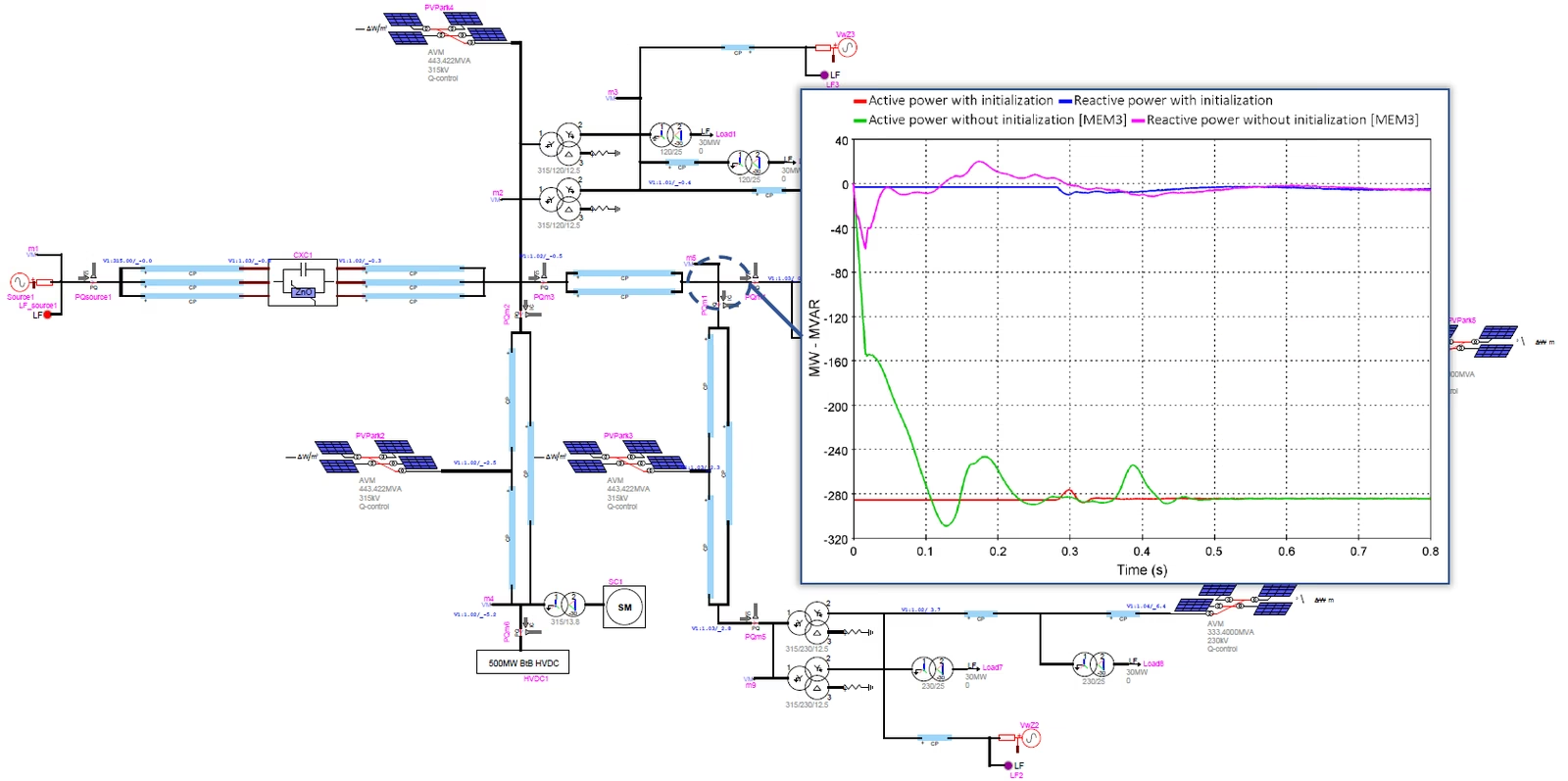
The contrast is stark when you compare the same case run with and without initialisation. Without it, the response opens with large oscillations, sits at the wrong operating point, takes a long time to settle, and sometimes never stabilises. With it, the transient is tiny, the model is immediately close to steady state, and the behaviour is stable from the first instant. A simple quality check follows: before applying a fault, switching event or setpoint change, the pre-disturbance traces should remain essentially flat — if they do not, the model is not properly initialised.

A large multi-machine EMT network (PV parks with average-value models, a back-to-back HVDC link, a synchronous machine and loads) with an overlaid plot of plant active and reactive power. With initialisation, the active power (red) and reactive power (blue) start flat at their steady-state values from t=0; without initialisation, the active power (green) plunges to nearly -300 MW with large, slowly decaying oscillations and the reactive power (magenta) swings before both settle only after about half a second. — Figure 1 — The same case with and without initialisation: the initialised run begins essentially at steady state, while the uninitialised run develops large artificial oscillations and settles only slowly.

Table 1 — Running with and without initialisation.
Aspect	Without Initialisation	With Initialisation
Start state	Zero or inconsistent	At the load-flow equilibrium
Initial transient	Large, artificial	Small, real events only
Settling	Long; may never settle	Immediate (a fraction of a second)
Weak grid	May diverge or show false instability	Stable
Computation	Seconds of run-up (heavy CPU)	Minimal
Parametric studies	Impractical	Practical

Section 4

Why it happens

The cause is simple: without initialisation the simulation starts from zero or inconsistent states. The capacitors are at the wrong voltage, the inductors at the wrong current, the converters at the wrong internal states, the PLL is not synchronised, and the controllers are not at equilibrium. From there the system has no choice but to self-adjust dynamically, and that self-adjustment is the artificial transient — fake oscillations, a long settling time, and, especially in weak grids, the risk of outright divergence. None of it corresponds to a real disturbance; it is the model finding the operating point it should have been given.

Section 5

Why it is critical for weak grids

This is where it bites hardest in renewable work. A weak grid has a low short-circuit ratio, so it is highly sensitive to disturbances and strongly coupled with the converter control. In a low-SCR system, a bad initial condition can act like an artificial disturbance and may trigger PLL oscillations, converter current-loop interaction or apparent SSCI behaviour. The danger is subtle: you may conclude that the system is unstable when in truth it is just badly initialised. A clean flat start helps distinguish real post-disturbance instability from numerical or modelling artefacts caused by inconsistent initial states — so in weak-grid studies it is not a nicety, it is what keeps the conclusion honest.

Bad init looks like instability

In a weak grid, a poor initialisation can produce exactly the oscillations you would expect from a genuine instability. Always rule out initialisation before declaring a system unstable.

Section 6

Initialisation is the equilibrium of a nonlinear system

Conceptually, initialisation is more than a load flow: it is finding the equilibrium of a nonlinear differential-algebraic system. The goal is a set of initial states for which nothing is changing — every derivative is zero:

\[ \left.\frac{d\mathbf{x}}{dt}\right|_{t=0} = \mathbf{0}, \qquad \mathbf{f}(\mathbf{x}_0,\mathbf{u}_0) = \mathbf{0} \]

\(\mathbf{x}\): state vector: inductor currents, capacitor voltages, converter and controller states
\(\mathbf{u}_0\): inputs at the operating point (from the load flow)
\(\mathbf{x}_0\): the initial states sought, for which the system is at rest

The states must satisfy the network equations, the converter dq control, the PLL phase-locking, the current limits and the control loops all at once. That simultaneous equilibrium — not just the load-flow voltages — is what makes initialisation both difficult and valuable.

Section 7

What gets initialised

Mapping that equilibrium onto the model means setting states across every domain, not just the bus voltages. In plain terms, inductors need initial currents, capacitors need initial voltages, machines need their rotor and electrical states, converters need dc-link and control states, and the PLL needs a consistent angle and frequency:

Table 2 — What is initialised from the load-flow solution.
Domain	States Set from the Load Flow
Network	Inductor currents and capacitor voltages
Converters	Internal converter and dc-link states
Synchronisation	The PLL angle, aligned with the grid voltage
Controllers	PI memories, filter states, references and limiters
Machines	Field voltage, mechanical power and exciter states

The PLL in particular should start already locked to the steady-state grid-voltage angle and frequency; otherwise the converter shows an artificial synchronisation transient before the actual study event. With all of these consistent, the time-domain run starts with no artificial transient — only the events you actually apply.

Section 8

Saving computation, and enabling parametric studies

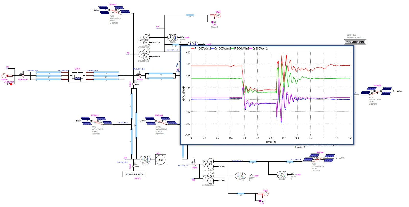
The practical payoff is large. Without proper initialisation a model may need seconds of simulated run-up just to settle — which can be minutes or hours of CPU — before any real study can begin. With it, only a small transient remains, a tenth to a few tenths of a second, so studies run far faster. Better still, the same initialisation can be reused across operating points, which is what makes parametric studies practical: initialise once, then run a fault for several conditions and compare.

The same EMT network with an overlaid plot of active and reactive power for two irradiance levels. At 1000 W/m2 the active power (red) starts flat near 290 MW; at 300 W/m2 it (green) starts flat near 180 MW; both reactive powers (blue and magenta) start near zero. Each run begins from a clean flat steady state, then the same fault is applied around 0.4 s and again near 0.65 s, so the responses at the two operating points are directly comparable. — Figure 2 — Initialise once, vary the operating point: faults applied at different irradiance levels, each starting from a clean flat start, so the responses are directly comparable without re-running a long settling.

Section 9

Flat start and the developer’s burden

All of this has a cost, and it falls on the model developer rather than the user. It is not enough to initialise the network voltages and the machine power; everything must be initialised — the filters, the transfer functions, the PI blocks, the limiters, the references and the internal memories of every controller. The network can be electrically consistent and the run still open with an artificial transient if the PI memories, filters, limiters, references or PLL states are not initialised to match. If even one important block starts from the wrong value, it will react at the next step and push the output off equilibrium, creating an artificial transient even though the output looked right at \(t=0\). That is why a clean flat start — the EMT run beginning directly at the steady-state operating point with no settling — is the product of deliberate, block-by-block work.

Section 10

Block-by-block backward initialisation

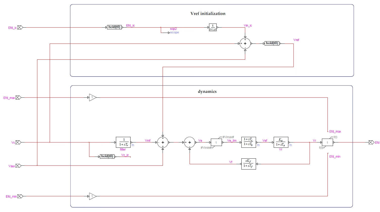
The standard technique is to work backward from the known output. Take the synchronous machine with an EXST1 exciter: the load flow fixes the terminal voltage and active power, from which the machine model determines the field voltage \(E_{fd}\) needed in steady state — the correct equilibrium output of the exciter. The task is then to make the controller produce exactly that \(E_{fd}\) at the first time step, with no transient, by initialising each block in turn so its stored state and its output are consistent. Where a block is a simple gain, this is just division:

\[ \text{gain: } y = K_a\,x \ \ \Rightarrow\ \ x_0 = \frac{y^{\ast}}{K_a}, \qquad y^{\ast} = E_{fd}\ \text{(from load flow)} \]

\(y^{\ast}\): the required steady-state output (the field voltage \(E_{fd}\))
\(K_a\): the exciter gain
\(x_0\): the internal signal (such as \(V_{ref}\)) set so the output is already correct

The known output is propagated backward, block by block: through a gain, divide by \(K_a\); through a dynamic block (filter, integrator), set its history state — not just its output — so the stored memory the solver uses is correct. A PI controller output depends not only on the present error but also on its stored integral state, so the integral memory must be set consistently with the required steady-state output. A limiter needs care: the initial operating point should normally sit inside the expected limiter range, unless the physical steady state is genuinely limited — if a limiter is already active at \(t=0\), that must be intentional and documented. The hold(t0) blocks force these calculated initial values at the first instant, and a small “h” on a signal marks that it is initialised. The final check is that the controller output is unchanged at the first time step: if it moves, some block’s stored state is still wrong. Continue until every block is consistent — and although the EXST1 exciter is the example here, the same block-by-block method applies to converter controls, PLLs, plant controllers, governors and HVDC controls.

The EXST1 exciter block diagram in EMTP, split into two regions. The upper Vref initialization region takes the initial field voltage Efd_ic through a hold(t0) and a 1/Ka gain to form Vref. The lower dynamics region is the running exciter: the voltage Vc through a filter 1/(1+sTr), a summing junction, a limiter, a lead-lag (1+sTc)/(1+sTb), the main gain Ka/(1+sTa), an output limiter between Efd_max and Efd_min, and the rate feedback sKf/(1+sTf), with hold(t0) blocks setting the initial states so the output Efd sits at equilibrium from the first step. — Figure 3 — The EXST1 exciter initialised block by block: the field voltage \(E_{fd}\) comes from load flow, and the internal references and states are set backward through the controller so the output is at equilibrium from the first step.

Section 11

A requirement for manufacturer models

The same approach applies far beyond the exciter — to governors, DFIG and Type-4 converter controls, plant controllers, the PLL, HVDC controls, and the OEM white-box and black-box renewable models. The general rule is that every dynamic subsystem must be initialised internally from the steady-state operating point. Because converter-based plants carry many nested loops — the PLL, the dq current controllers, the dc-link controller, the reactive/voltage controller, the plant controller, the protection logic, the pitch or MPPT loops — a model that is not initialised correctly can hunt, oscillate, drift or collapse in weak-grid conditions. That is why a clean flat start from load flow should be treated as a requirement of model quality, asked for explicitly when commissioning any manufacturer EMT model — good fault dynamics alone are not enough. Not every legacy or black-box model can expose its internal states for perfect initialisation, though; where that is the case, the limitation should be documented rather than hidden.

Ask for it

When receiving an OEM model, request evidence that it can initialise from the specified operating point without a long settling run or artificial start-up oscillation. A model that only reproduces fault dynamics but cannot flat-start will make studies slow and weak-grid cases unreliable.

Section 12

Key points

Start at equilibrium, block by block

An EMT run should start from a consistent steady state — the load-flow equilibrium, not zero or arbitrary states.
The load flow must be mapped to the EMT states: inductor currents, capacitor voltages, converter, PLL and controller states.
Zero or inconsistent states create artificial transients — long settling and, in a weak grid, false instability that is merely bad initialisation.
Every controller block must be initialised, backward from its known steady-state output (gains, filters, PI memories, limiters, references, history).
A clean flat start is essential for weak-grid and manufacturer-model studies, and should be treated as a model-quality requirement.

For the specific cases, see the DFIG and synchronous-machine load-flow initialisation guides; for why it matters most in weak grids, the EMT-versus-RMS guide.

References

EMTP® Documentation and Application Notes. Powersys / EMTP®.

Built on EMTP® · Expert spotlight

Henry Gras

Chief Operating Officer, PGSTech · Montréal, Canada

Henry Gras delivers the EMTP® University course “EMT Simulation and Analysis of Large-Scale Power Systems with Renewables” and works daily with the tool this article is written around.

Henry is based in Montréal, where he is Chief Operating Officer of PGSTech, the company responsible for EMTP® engineering services, commercialisation and continuing software development. He holds a master’s degree from Polytechnique Montréal, where he worked on electrical-machine research, and previously completed an engineering degree at École Centrale de Lyon in France.

Readers who want a structured programme on EMT simulation of large-scale power systems with renewables will find his EMTP® University course an excellent next step.

Henry’s technical expertise covers electromagnetic transient simulation, renewable-energy integration, power-system modelling, electrical machines, protection and specialist transient studies including TRV, transformer energisation, ferroresonance, insulation coordination and power quality.

Part 30 Reading now

EMT Initialisation and Flat Start

Load-flow initialisation and block-by-block controller states for a clean flat start.

Series progress 30 of 30

All thirty parts

Explore more technical guides

You have reached the end of the renewable-energy EMT modelling series. Browse the full APS technical library for more power-system study guides.