Renewable Modelling · DSC Sequence Extraction

DSC Sequence Extraction and the SSCI Parameter Mask in EMTP®: DSRF, Coupled Feed-Forward and Filters

The DSC implementation guide showed the four current loops and the decoupled solver. This page goes one layer deeper: how the positive- and negative-sequence currents are actually extracted from the measured signals, and why the EMTP® control mask exposes so many parameters. The extraction uses a Clarke transform, a double synchronous reference frame and careful filtering; the feed-forward is kept coupled in the αβ frame; and the long list of mask options exists because sub-synchronous control interaction and weak-grid behaviour depend on the measurement filters, the PLL and the sampling — not just the PI gains.

Reading time ≈ 20 min · DSRF extraction, feed-forward & SSCI mask

The DSC implementation guide covered the four current loops and the decoupled solver. This page sits one layer beneath them: the signal processing that runs before the PI regulators, and the parameters that shape it. Under unbalance the measured current is a mix of positive and negative sequence, so the controller must first separate the two; that separation uses a Clarke transform, a double synchronous reference frame and careful filtering. The same implementation layer is also why the EMTP® control mask exposes so many options — because, in weak grids and sub-synchronous control interaction (SSCI) studies, those filtering and timing details matter as much as the PI gains.
Abbreviations used on this page
DSCDecoupled sequence control
DSRFDouble synchronous reference frame
GSCGrid-side converter
\(\alpha\beta\)Stationary two-axis frame
d–qRotating reference frame
\(C\)Clarke transformation matrix
\(P\)Park transformation matrix
LPFLow-pass filter
PLLPhase-locked loop
SSCISub-synchronous control interaction
FRTFault ride-through
PIProportional–integral controller
PWMPulse-width modulation
\(2\omega\)Twice fundamental frequency (100 Hz on a 50 Hz system)
ac / dcAlternating / direct current
EMTP®Electromagnetic Transients Program
EMTElectromagnetic transient (time domain)
Key idea
  1. DSC’s implementation layer is signal processing before the PI: the measured current goes Clarke → \(\alpha\beta\), is projected into positive- and negative-sequence rotating frames, low-pass filtered and cross-term-cancelled to give clean \(i_{dq}^{+}\) and \(i_{dq}^{-}\).
  2. The low-pass filters are the decoupling: positive sequence is dc in the positive frame while negative sequence appears at \(2\omega\) there (and vice versa), so the LPF keeps the dc and rejects the contamination. The angle comes from a double synchronous reference frame (DSRF), because an ordinary PLL is disturbed by the negative sequence under unbalance.
  3. The feed-forward terms are kept coupled — \((\omega L_{choke}\,i_{qg}+v_{d\text{-}choke})\) and \((-\omega L_{choke}\,i_{dg}+v_{q\text{-}choke})\) — and added to the PI outputs in the stationary \(\alpha\beta\) frame, because the physical choke / grid voltage drop is genuinely coupled.
  4. The mask exposes many parameters (PWM / sampling, measurement-filter type / order / cut-off, control mode, FRT thresholds, current limits, external \(R\)/\(X\)) because SSCI and weak-grid behaviour depend on the filters, the PLL and the sampling — not only the PI and PLL gains.
Key terms used on this page
01DSRF
Double synchronous reference frame: two frames (positive and negative) used for angle tracking and sequence work under unbalance.
02Sequence extraction
Separating the measured current into clean positive- and negative-sequence dq components.
03Clarke transform
\(C\): maps three-phase abc quantities to the stationary two-axis \(\alpha\beta\) frame.
04Park transform
\(P\): rotates \(\alpha\beta\) into a synchronous dq frame; \(P^{+1}\) for positive, \(P^{-1}\) for negative.
05Low-pass filter
Keeps the dc (own-sequence) part and rejects the \(2\omega\) contamination from the other sequence.
06Cross-term cancellation
Reconstructing and subtracting each sequence’s leakage into the other’s frame.
07Coupled feed-forward
Compensation kept in coupled physical form and applied in \(\alpha\beta\), not split into one balanced dq frame.
08SSCI
Sub-synchronous control interaction: converter–grid oscillation driven by control dynamics, esp. in weak grids.
09Measurement filter
The input filter (type, order, cut-off); it adds lag and phase shift that enter the closed-loop dynamics.
10DSRF PLL
A PLL using the double synchronous reference frame to track the angle cleanly under unbalance.
11Apparent impedance
The converter’s frequency-domain behaviour seen by the grid; shaped by the PLL and filters.
12External system equivalent
An \(R\)/\(X\) representing the grid strength the converter is connected to.

Section 1

The implementation layer of DSC

Behaviour under unbalance is not decided by the PI loops alone. It depends on the sequence-extraction method, the PLL structure, the measurement filters, the sampling and the current-priority settings. That is exactly why the model exposes so many parameters in its mask: for research and SSCI work these implementation details are not secondary. This page works through the two halves of that layer — how the sequences are extracted, and what the mask lets you set. Throughout, sub-synchronous control interaction (SSCI) means an interaction between the converter controls and the network impedance at frequencies below the fundamental that can reduce damping or excite growing oscillations — and it is unusually sensitive to exactly these implementation details.

Beyond the control law

Converter control under unbalance is also about how the signals are processed: sequence extraction, PLL, filters, sampling, feed-forward placement and priority logic. In weak-grid / SSCI work those details can change the result significantly.

Section 2

Mixed sequences in the measured current

When the grid is unbalanced, the measured three-phase current \(i_{abc}\) contains both a positive-sequence component, whose phasor rotates forward at \(+\omega\), and a negative-sequence component, whose phasor rotates backward at \(-\omega\). A single ordinary dq transformation can lock to only one of them — say the positive-sequence angle \(+\omega\). In that frame the positive sequence stands still and becomes a clean dc quantity, but the negative sequence, turning the opposite way, is seen rotating at \(-2\omega\) and appears as a double-frequency (\(2\omega\)) oscillation on the dq signals — 100 Hz on a 50 Hz system. A PI regulator cannot hold a moving target to zero error, so a single dq frame simply cannot produce clean references under unbalance. That is why the first step of DSC is not control at all; it is separation: take \(i_{abc}\) and produce clean positive- and negative-sequence dq currents for the four loops to act on.

Section 3

The extraction chain

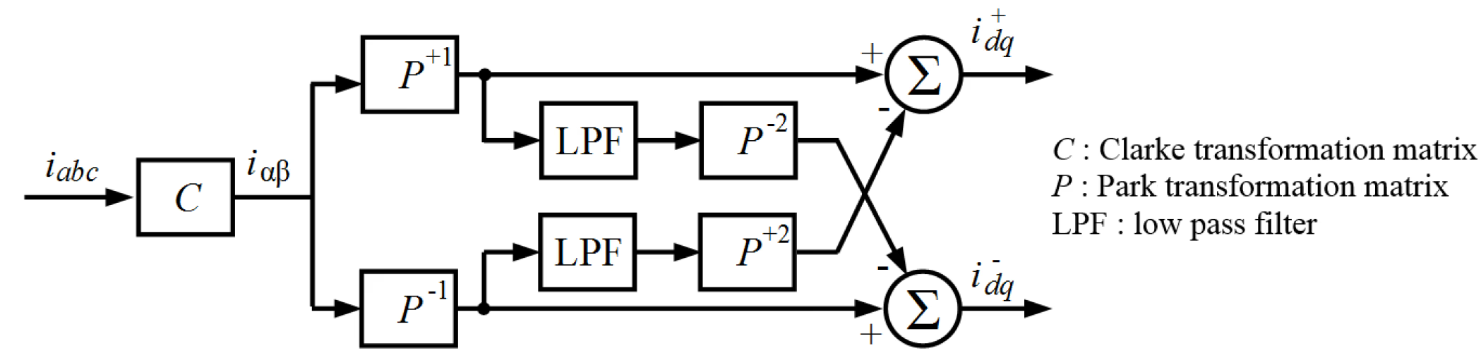
The separation runs as a short chain. The current is first taken to the stationary \(\alpha\beta\) frame with the Clarke transform, then projected into a positive-sequence rotating frame and a negative-sequence rotating frame:

\[ i_{\alpha\beta} = C\,i_{abc}, \qquad i_{dq}^{+} = P^{+1}\,i_{\alpha\beta}, \qquad i_{dq}^{-} = P^{-1}\,i_{\alpha\beta} \]
\(i_{abc}\)
measured three-phase current (mixed positive and negative sequence)
\(i_{\alpha\beta}\)
the same current in the stationary two-axis (Clarke) frame
\(C\)
Clarke transformation matrix (abc → \(\alpha\beta\))
\(P^{+1},\ P^{-1}\)
Park transforms into the positive- (\(+\omega\)) and negative- (\(-\omega\)) sequence frames
\(i_{dq}^{+},\ i_{dq}^{-}\)
positive- and negative-sequence dq currents (after filtering and cross-term cancellation)

Each projected frame is still contaminated by the other sequence, so low-pass filters and a cross-term reconstruction are applied before the outputs are clean.

Sequence extraction by the decoupling method: the measured current i_abc passes through a Clarke transform to the alpha-beta frame, is projected into positive- and negative-sequence rotating frames, low-pass filtered, and has a reconstructed cross-term subtracted, giving clean positive- and negative-sequence dq currents.
Figure 1 — Sequence extraction by the decoupling method. The Clarke transform takes \(i_{abc}\) to \(i_{\alpha\beta}\), projected into positive- and negative-sequence frames; a low-pass filter keeps each sequence’s dc part while a reconstructed cross-term is subtracted, giving the clean \(i_{dq}^{+}\) and \(i_{dq}^{-}\) currents.

Section 4

The filters do the separating

The low-pass filters in that diagram are not ordinary noise filters — they are part of the extraction mechanism. When the positive-sequence current is observed in the positive synchronous frame it becomes a dc quantity, while the negative-sequence current appears there as a double-frequency oscillation. In the negative frame it is the other way round: negative sequence is dc, positive sequence is oscillatory. So low-pass filtering keeps the dc (own-sequence) part and rejects the oscillatory contamination from the other sequence. That, together with reconstructing and subtracting the cross-terms, is the mathematical basis of the decoupling method.

There is a genuine trade-off in the filter cut-off: a lower cut-off rejects the \(2\omega\) contamination more completely but slows the extraction and adds phase lag, while a higher cut-off responds faster but lets more of the other sequence leak through. “Reconstructing the cross-term” simply means the estimator rebuilds what the opposite sequence would look like in this frame and subtracts it, instead of leaning on the filter alone. Neither step is perfect — a little residual coupling and a little delay always remain — which is one reason the extraction settings themselves influence stability.

Section 5

The DSRF and the PLL

The rotating-frame angle \(\theta\) — the tracked grid-voltage angle, whose rate of change \(\omega = \mathrm{d}\theta/\mathrm{d}t\) is the grid frequency — is derived from a double synchronous reference frame (DSRF), positive- and negative-sequence frames working together, rather than a single ordinary PLL. The reason is the same one that makes extraction necessary: a normal PLL assumes a mostly balanced positive-sequence voltage, but under unbalance the positive and negative sequences mix, the phase estimate oscillates, and the dq variables get polluted. So with DSC the angle-tracking mechanism itself must understand the sequences and their separation, which is why a DSRF (or equivalent decoupled) PLL is used. The angle tracking is no longer a separate, simple step — it is part of the sequence machinery.

Section 6

Feed-forward kept in coupled form

A subtle implementation choice concerns the feed-forward compensation. In ordinary balanced control those terms — choke reactance, measured voltage, dq coupling — are applied in a single dq frame. Under DSC they are instead kept in coupled form and added to the PI regulator outputs in the stationary \(\alpha\beta\) frame:

\[ \big(\,\omega L_{choke}\,i_{qg} + v_{d\text{-}choke}\,\big) \qquad\text{and}\qquad \big(\,-\omega L_{choke}\,i_{dg} + v_{q\text{-}choke}\,\big) \]
\(L_{choke}\)
the converter choke (filter) inductance; \(\omega L_{choke}\) is its reactance at grid frequency
\(i_{dg},\ i_{qg}\)
the grid-side converter dq currents
\(\omega L_{choke}\,i\)
the dq cross-coupling through the choke reactance
\(v_{d\text{-}choke},\ v_{q\text{-}choke}\)
the measured choke / terminal voltage components

The opposite signs on the two cross-terms — \(+\omega L_{choke}\,i_{qg}\) on the d-axis, \(-\omega L_{choke}\,i_{dg}\) on the q-axis — are the standard dq cross-coupling convention that cancels the choke’s reactive coupling. They are kept coupled and added in the stationary \(\alpha\beta\) frame because the physical choke and grid-voltage drop is fundamentally coupled — forcing it too early into one idealised balanced dq compensation introduces errors.

So the robust implementation applies the compensation where the real voltage–current relationship is represented properly, and lets the decoupled sequence loops work on top of it. This is the kind of detail that separates a research- or OEM-grade implementation from a textbook one.

Section 7

What the \(c2\) and \(s2\) terms mean

A small notational point worth settling, because it says what the negative-sequence current references — the quantities the decoupled loops and the mask ultimately shape — are actually for. Active power under unbalance is not constant; it has a mean plus a part that pulses at twice the grid frequency, written \(p(t)=P_0+P_{c2}\cos 2\omega t+P_{s2}\sin 2\omega t\). Here \(P_0\) is the average (dc) power the dc link must balance, while \(P_{c2}\) and \(P_{s2}\) are the cosine and sine coefficients of the \(2\omega\) ripple: \(P_{c2}\) scales the \(\cos 2\omega t\) part and \(P_{s2}\) the \(\sin 2\omega t\) part, with the “2” marking the second harmonic. The reactive power \(q(t)\) has the same structure, with its own \(Q_0\), \(Q_{c2}\) and \(Q_{s2}\). Reading the subscripts this way — \(c\) for cosine, \(s\) for sine, 2 for \(2\omega\) — is enough to read that decomposition wherever it appears. The point for this page is that the negative-sequence references are chosen precisely to drive selected coefficients to zero — \(P_{c2}\) and \(P_{s2}\) for constant active power, or the reactive pair for constant reactive power; the full \(p(t)\)/\(q(t)\) reference equations are set out in the DSC implementation guide.

Section 8

The control-parameter mask

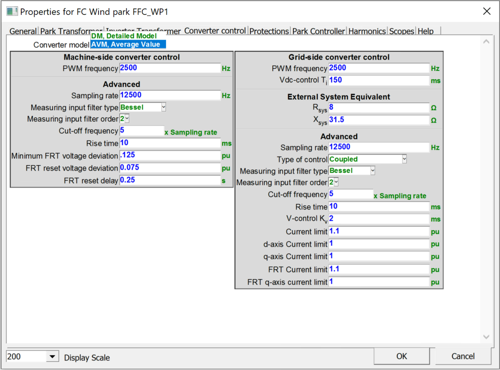
The other half of the implementation layer is what the user can set. In EMTP® a device’s mask is the parameter-entry dialog that sits over the underlying model — the fields an engineer fills in without editing the internal control diagram. The converter-control mask exposes a large set of these parameters, on both the machine-side and grid-side converters, with example values shown below.

Table 1 — Representative grid-side converter-control mask parameters (example values).
GroupParameterExampleWhat It Shapes
TimingPWM frequency2500 HzConverter switching and harmonic content
TimingSampling rate12500 HzDigital control timing and delay
TimingRise time10 msCurrent-loop bandwidth
FilterMeasuring input filter typeBesselMeasurement phase / delay — affects SSCI
FilterFilter order / cut-off2 / cut-off ≈ sampling ÷ 5Roll-off and phase lag of the measurement
Loops\(V_{dc}\)-control \(T_i\)150 msdc-voltage loop response speed
LoopsV-control \(K\)2Outer voltage-loop sensitivity
ModeType of controlCoupledSequence / decoupling mode
GridExternal system equivalent\(R_{sys}=8\,\Omega\), \(X_{sys}=31.5\,\Omega\)Grid strength (short-circuit level) the converter sees
LimitsCurrent limits (total / d / q / FRT / FRT-q)1.1 / 1 / 1 / 1.1 / 1 puCurrent-priority envelope (normal and FRT)

The values sit on the converter’s own bases: the current limits are per-unit on the converter’s rated-current (MVA) base, the times are in milliseconds, and \(R_{sys}\) and \(X_{sys}\) are in ohms referred to the connection voltage. Those last two set the Thévenin impedance the converter works against and therefore the short-circuit ratio: a larger \(X_{sys}\) means a weaker grid, a lower short-circuit ratio and, usually, more SSCI risk.

The converter-control parameter mask of the full-converter wind-park model, exposing machine-side and grid-side PWM and sampling, measurement-filter type, order and cut-off, rise time, control mode, FRT thresholds, the external system equivalent R_sys and X_sys, and the current limits.
Figure 2 — The converter-control parameter mask of the full-converter wind-park model. It groups the settings that shape the dynamic response: timing (PWM, sampling, rise time), measurement filters, the control mode and PLL, the current limits and FRT thresholds, and the external-grid equivalent \((R_{sys},X_{sys})\) — the parameters an SSCI or weak-grid study needs to set.

Section 9

Why so many parameters: SSCI and weak grids

The reason for all those options is practical. A great deal of research has gone into sub-synchronous control interaction, and the finding is that it is not only the PLL that matters but also the measurement-filter type, the filter order, the cut-off frequency, the sampling rate, the control mode and the current limits. Textbook explanations tend to focus on the PI gains and the PLL gains, but in real converter-stability work these “small” implementation details strongly affect damping, resonance, SSCI behaviour and weak-grid interaction. A converter’s frequency response depends on the complete time-domain control representation, so an SSCI assessment must respect the actual implemented control structure — which is why the mask gives that research freedom. None of these settings creates SSCI on its own; they let the model represent the real converter and grid closely enough that a genuine interaction, if the physical system has one, appears in the simulation instead of being hidden by an over-idealised control block.

Section 10

Why measurement filters matter for SSCI

Measurement filters have a real impact on SSCI, for a simple reason: every filter introduces lag, phase shift, attenuation and delay. In a tightly coupled converter–grid system those directly affect loop stability, effective damping, the shape of the converter’s impedance and its tendency to oscillate. So a measurement filter is not just signal cleanup — it is part of the closed-loop dynamics. That is why the mask lets you choose the filter type, order and cut-off frequency: they are genuine stability-shaping parameters, not cosmetic ones.

Order and cut-off act differently. A higher order gives a sharper roll-off but more phase lag near the cut-off; a lower cut-off removes more high-frequency content but delays the measurement more. The sampling rate is a separate effect again — it sets the control-update delay and the digital phase lag independently of the analogue filter. And sampling should not be confused with the PWM (switching) frequency: PWM sets how often the converter switches and where the switching harmonics land, whereas sampling sets how often the controller reads its inputs and updates its outputs. The two are often related in a model but are physically distinct.

Section 11

Why the PLL matters for SSCI

The PLL has a strong impact too. It affects angle tracking, the effective dq transformation, the converter’s apparent impedance and its low-frequency dynamic coupling with the network. In impedance terms, PLL dynamics can contribute negative damping, shape impedance resonances and drive sub-synchronous interaction. That is why, in modern converter-stability work, PLL design is often one of the first things checked in a weak-grid study — and why the model exposes the parameters that set it.

The mechanism is this: the PLL estimates the grid angle from the terminal voltage, but that voltage is itself moved by the converter’s own current flowing through the grid impedance. At sub-synchronous frequencies the PLL’s finite bandwidth turns that feedback into a frequency-dependent term in the converter’s apparent impedance — and over a band of frequencies that term can behave like a negative resistance, which is exactly what sustains an oscillation. It also helps to keep two ideas apart: a weak grid is simply one with a high source impedance (a low short-circuit ratio); SSCI is a specific sub-synchronous oscillation that a weak grid, or a series-compensated line, makes far more likely. The weak grid is the condition; SSCI is one of the failures it can produce.

  • Set the external \(R_{sys}\)/\(X_{sys}\) to the real short-circuit level, and its credible range, rather than a strong-grid default.
  • Use the PLL, filter and sampling settings that match the actual firmware, not idealised placeholders.
  • Sweep the band of interest with an impedance or frequency scan and check the damping across the sub-synchronous range.
  • Confirm the result stays stable over the full range of grid strength, not at a single operating point.

Section 12

Many options, not clutter

Not all of these parameters are needed for ordinary use — a standard study may only touch a small subset. But for research, OEM benchmarking, SSCI studies, weak-grid studies and control-sensitivity work, the extra options become very valuable. So the abundance is not clutter: it reflects the fact that a converter’s dynamic interaction with the network depends on many implementation details, and a faithful study needs to be able to set them.

The questions to ask

When someone says “we added negative-sequence control”, the informed questions are: how are the sequences extracted, what PLL is used, what filters, where is the feed-forward applied, and how are the cross-terms cancelled?

Section 13

Key points

The signal layer is as important as the control law

Under unbalance, DSC first separates the measured current: a Clarke transform to \(\alpha\beta\), projection into positive- and negative-sequence frames, low-pass filtering and cross-term cancellation give clean \(i_{dq}^{+}\) and \(i_{dq}^{-}\). The filters are part of the method (own-sequence dc kept, other-sequence \(2\omega\) rejected); the angle comes from a double synchronous reference frame because a single ordinary PLL is disturbed by the negative sequence and its estimate oscillates at double frequency; and the feed-forward terms are kept coupled and applied in the stationary \(\alpha\beta\) frame because the physical choke drop is coupled. The EMTP® mask exposes a long list of parameters — PWM and sampling, measurement-filter type / order / cut-off, control mode, rise time, FRT thresholds, current limits and an external \(R\)/\(X\) — because sub-synchronous control interaction and weak-grid behaviour are shaped by the measurement filters, the PLL and the sampling, not just the PI gains. For the loops these feed and the concept behind them, see the DSC implementation and current-loop guides.

References

References

  1. EMTP® Documentation and Application Notes. Powersys / EMTP®.
Built on EMTP® · Expert spotlight
Portrait of Henry Gras, Chief Operating Officer of PGSTech

Henry Gras

Chief Operating Officer, PGSTech · Montréal, Canada

Henry Gras delivers the EMTP® University course “EMT Simulation and Analysis of Large-Scale Power Systems with Renewables” and works daily with the tool this article is written around.

Henry is based in Montréal, where he is Chief Operating Officer of PGSTech, the company responsible for EMTP® engineering services, commercialisation and continuing software development. He holds a master’s degree from Polytechnique Montréal, where he worked on electrical-machine research, and previously completed an engineering degree at École Centrale de Lyon in France.

Readers who want a structured programme on EMT simulation of large-scale power systems with renewables will find his EMTP® University course an excellent next step.

Henry’s technical expertise covers electromagnetic transient simulation, renewable-energy integration, power-system modelling, electrical machines, protection and specialist transient studies including TRV, transformer energisation, ferroresonance, insulation coordination and power quality.

Thirty-Part Technical Series

EMTP® Renewable Energy Modelling

A thirty-part guide to modelling wind, PV and full-converter plant in EMTP® — sources and turbines, converter and plant control, sequence control under faults, protection, and weak-grid and SSCI stability.

Part 14 Reading now

DSC Sequence Extraction and the SSCI Mask

How the sequences are actually separated — the DSRF, coupled feed-forward, filter choices and their effect on SSCI sensitivity.

Series progress 14 of 30