Renewable Modelling · DFIG Wind Park

DFIG Wind Park Modelling in EMTP®: Architecture, Load Flow and Initialisation

A wind park is not a single machine but a layered system — blades and a flexible shaft, a doubly-fed induction generator (DFIG), a back-to-back converter, local and plant-level controllers, a collector network and a grid transformer. EMTP® packages all of this into one model and, crucially, represents it at the level of detail each study needs rather than in a single universal form. This guide reads the architecture layer by layer, and shows how the model is initialised so an electromagnetic-transient (EMT) simulation starts from the correct operating point.

Reading time ≈ 28 min · DFIG architecture, load flow & initialisation

A modern wind park looks like a single line on a network diagram, but behind that line is a layered machine — from rotating blades on a flexible shaft, through a doubly-fed induction generator (DFIG, Type-3) and its power-electronic converter with a dc (direct-current) link and protection, to the medium-voltage collector cables and the transformer stages up to the grid. The generic DFIG wind-park model in EMTP® (the Electromagnetic Transients Program) packages all of this into one component. The recurring theme of this guide is that the same plant is shown to each study at a different level of detail. The sections below read the architecture layer by layer, then show briefly how the plant is reduced to a load-flow injection and seeded so a time-domain simulation starts from the correct operating point — the detailed load-flow and initialisation workflow has its own dedicated guide.

Abbreviations used on this page

DFIGDoubly-fed induction generator (Type-3)

EMTElectromagnetic transient

EMTP®Electromagnetic Transients Program

WT / WPWind turbine / wind park

WPCWind-park controller

RSCRotor-side converter

GSCGrid-side converter

IGInduction (asynchronous) generator

POIPoint of interconnection

OLTCOn-load tap changer

PQSpecified active / reactive power bus

PVSpecified-power, controlled-voltage bus

dcDirect current

d–qDirect–quadrature rotating frame

FRTFault ride-through

MPPTMaximum-power-point tracking

\(\pi\)-circuitLumped R–L–C line / cable equivalent

\(C_p\)Aerodynamic power coefficient

Key idea

A wind park is one model with several faces: the same plant is represented at the level of detail each study needs, and the engineer selects that representation rather than relying on a single “universal” model.
The model is layered: aerodynamic turbine → two-mass shaft → DFIG electrical system (generator, back-to-back converter, dc link, protection, turbine transformer) → local wind-turbine (WT) control → equivalent collector grid → park transformer → supervisory wind-park (WP) control → initialisation.
In a DFIG the stator connects directly to the grid while the rotor is fed through a partially-rated back-to-back converter. The rotor-side converter shapes machine power and stator-side reactive support; the grid-side converter holds the dc-link voltage.
For load flow the whole plant collapses to a PQ injection — active power set by the wind, reactive power by the control mode. A load-flow-constrained initialisation source then seeds the detailed EMT model so it starts without artificial transients.

Key terms used on this page

01DFIG (Type-3)

Wound-rotor induction generator with the stator on the grid and the rotor fed by a converter, allowing variable-speed operation around synchronous speed.

02Back-to-back converter

Two voltage-source converters sharing a dc link — the rotor-side and grid-side converters — that exchange the rotor slip power with the grid.

03Rotor-side converter (RSC)

Feeds the rotor windings; controls the generator active power (torque) and the stator-side reactive power or voltage.

04Grid-side converter (GSC)

Connects the dc link to the grid; regulates the dc-link voltage and can provide a limited amount of reactive support.

05dc link

The capacitor-buffered dc stage between the two converters; its voltage is the energy buffer the GSC must keep constant.

06Crowbar / chopper

Rotor and dc-link protection that absorbs energy and shields the converter during grid faults and dc over-voltage.

07Two-mass shaft

Turbine inertia and generator inertia joined by a finite shaft stiffness and damping — needed to reproduce drive-train torsional behaviour.

08Power coefficient \(C_p\)

Fraction of the wind’s kinetic power captured by the rotor; a function of tip-speed ratio and blade pitch.

09Wind-park controller (WPC)

Supervisory plant controller that meets the grid-code targets at the POI and dispatches set-points to the turbines.

10Equivalent collector grid

A reduced π-circuit (or short feeder set) that reproduces the impedance and charging of the real medium-voltage cable network.

11Aggregated model

One scaled equivalent turbine standing in for many identical units, with ratings and impedances scaled by the number aggregated.

12Initialisation source

A load-flow-constrained source that imposes the steady operating point so the detailed model starts in balance, free of start-up transients.

Section 1

One model, many studies

The single most useful idea to hold onto is that a wind-park model is not one fixed thing. The plant that appears as a full dynamic model in an electromagnetic-transient (EMT) study appears as a single algebraic power injection in a load-flow study, and as a frequency-dependent impedance in a harmonic study. None of these is “the” model; each is the appropriate face of the same plant for a particular question. The engineering decision, exactly as for any other power-system component, is to choose the representation that contains the physics controlling the result — and to leave out the physics that does not.

This matters in practice because the detailed EMT representation is expensive and easy to mis-initialise, while the load-flow representation is trivial but says nothing about dynamics. A generic DFIG model is built to provide both: a compact load-flow behaviour for setting the operating point, and a full dynamic behaviour for the transient itself, linked so that the second starts from the first.

The governing question

What does this study need from the wind park — a steady power injection, a frequency response, or a full dynamic response to a disturbance? The answer fixes the level of detail, and everything else follows.

Section 2

The model in layers

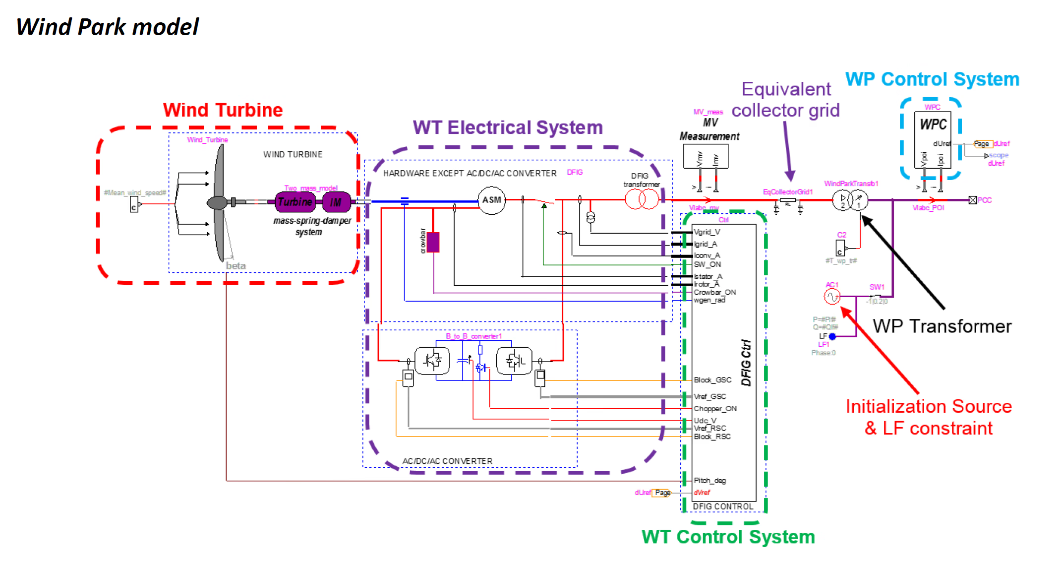
It helps to read the model as a stack of layers, each handing physical quantities to the next. The wind drives an aerodynamic rotor, which delivers mechanical torque through a flexible shaft to the induction generator. The generator’s rotor is fed by a back-to-back converter with its own dc link and protection; its stator and the converter’s grid side join at the turbine transformer. A local turbine controller sets converter references; a supervisory wind-park controller coordinates the turbines to meet targets at the point of interconnection. The turbines feed an equivalent collector grid, which feeds the park transformer and finally the grid. Beneath all of this sits the initialisation machinery that places the plant at its steady operating point before any disturbance is applied.

EMTP schematic of the generic DFIG wind-park model: the wind turbine, the DFIG electrical system with its back-to-back converter and crowbar, the DFIG control, MV measurement, the equivalent collector grid and the wind-park transformer through to the point of interconnection (POI), plus the wind-park controller (WPC) and an initialisation source imposing the load-flow constraint. — Figure 1 — The generic DFIG wind-park model in EMTP®: the wind turbine (aerodynamics and two-mass shaft) drives the DFIG electrical system — induction generator, crowbar, back-to-back RSC/GSC converter and turbine transformer — under its DFIG control; the turbine then feeds the MV measurement, the equivalent collector grid and the wind-park transformer through to the point of interconnection (POI), while the wind-park controller (WPC) sits above and an initialisation source imposes the load-flow constraint.

Section 3

The wind turbine: aerodynamics and shaft

The first layer converts wind into mechanical torque. The aerodynamic block computes the power captured from the wind as a fraction of the kinetic power passing through the rotor disc. That fraction, the power coefficient \(C_p\), depends on the tip-speed ratio \(\lambda=\omega_t R/v\) (how fast the blade tips move relative to the wind) and on the blade pitch angle \(\beta\). Below rated wind speed the controller holds \(\beta\) near its optimum and tracks the speed that maximises \(C_p\); above rated wind speed it pitches the blades to shed power and protect the machine.

\[ P_t = \tfrac{1}{2}\,\rho\,A\,v^{3}\,C_p(\lambda,\beta), \qquad \lambda=\frac{\omega_t R}{v} \]

\(P_t\): mechanical power captured by the rotor (W)
\(\rho\): air density (kg/m³)
\(A=\pi R^{2}\): swept area of the rotor (m²)
\(R\): rotor radius (m)
\(v\): wind speed at the rotor (m/s)
\(C_p(\lambda,\beta)\): power coefficient — a dimensionless function of tip-speed ratio and pitch
\(\lambda\): tip-speed ratio (blade-tip speed ÷ wind speed), dimensionless
\(\beta\): blade pitch angle (degrees)
\(\omega_t\): turbine (rotor) angular speed (rad/s)

The cube of wind speed is why a small change in wind makes a large change in power, and why the controller must continuously retune \(\lambda\) and \(\beta\) to stay on the best operating point.

The captured power reaches the generator through the drive train. For slow studies a single rigid mass is enough, but for transient work the shaft is represented as two masses — the large turbine inertia and the smaller generator inertia — joined by a finite stiffness and damping. The turbine speed \(\omega_t\) used above and the generator speed are therefore distinct state variables, coupled through the shaft (and the gearbox ratio) rather than locked together. This matters during grid faults: the electrical torque at the generator can change within milliseconds, while the large mechanical inertia of the turbine cannot follow instantly, so the shaft twists and the drive train oscillates torsionally — an effect a single-mass shaft cannot reproduce. The two-mass shaft is written as a small set of state equations linking the two speeds and the twist angle between them.

Section 4

The DFIG electrical system

The defining feature of a Type-3 turbine is that the generator is doubly fed: its stator is connected directly to the grid (through the turbine transformer) while its wound rotor is fed by a converter. By injecting a controllable voltage into the rotor at slip frequency, the converter lets the machine run efficiently across a band of speeds around synchronous — typically a few tens of per cent either side — without the converter ever having to carry the full machine power.

That is the commercial point of the topology. The converter only processes the rotor slip power — the power associated with the rotor circuit when the machine runs away from synchronous speed (broadly, the slip fraction of the air-gap power). Because it handles only this slip power, the converter is rated for a fraction of the turbine rating — commonly around a quarter to a third — though the exact figure depends on the permitted speed / slip range and the OEM design and should not be treated as a universal number. The electrical layer therefore contains: the induction generator itself (stator and rotor windings, represented in the usual d–q (direct–quadrature) form), the back-to-back converter on the rotor, the dc link between the two converter stages, the crowbar and dc-chopper protection, and the turbine transformer that ties stator and converter to the medium-voltage collector network.

Why it is “partially rated”

The stator carries the bulk of the power straight to the grid; the converter only handles the rotor slip power. A smaller converter means lower cost and losses — but it also means the converter has limited headroom, which is exactly why fault protection (crowbar, chopper) is part of the electrical model.

Section 5

Rotor-side and grid-side converters

The back-to-back converter is two voltage-source converters sharing one dc link, and the two have distinct jobs.

The rotor-side converter (RSC) faces the machine rotor. Working in a stator-flux-oriented frame, it controls the generator’s active power (and hence electromagnetic torque) through one current component and the stator-side reactive power or voltage through the other. This is the converter that actually shapes how much power the turbine produces and how it supports voltage.
The grid-side converter (GSC) faces the grid. Its first duty is to keep the dc-link voltage constant by passing the rotor slip power on to the grid; whatever the RSC pushes into or pulls out of the dc link, the GSC balances. It can also supply a limited amount of reactive power of its own, though the main reactive capability of the turbine comes from the stator via the RSC.

Between them sits the dc link, a capacitor that buffers the energy exchanged by the two converters; its voltage is the variable the GSC defends. When a grid fault drives large rotor currents, the crowbar short-circuits the rotor through a resistance to protect the RSC — but while it is engaged the RSC loses control and the machine momentarily behaves like a plain squirrel-cage induction generator. The dc resistive chopper plays a related but distinct role: it limits the dc-link over-voltage by dissipating excess energy. By keeping the dc bus within bounds the chopper can reduce the likelihood of crowbar operation in some events, but it does not replace the crowbar — it gives no protection against rotor over-current, so both are needed. On the grid side, a line inductor (choke) and an ac harmonic filter improve power quality and, as on the full-scale converter, help shape the converter’s impedance for harmonic and sub-synchronous interaction studies; how much filter detail is actually required depends on the study objective and on the OEM data available. Representing the protections and filters is essential for any fault-ride-through (FRT) or harmonic study — without them the converter model would see currents and voltages it could never survive in reality.

Section 6

The local WT control system

Each turbine has its own controller that turns high-level commands into converter and pitch actions. It contains the fast inner current loops of the RSC and GSC, the outer loops for power, dc-link voltage and reactive support, the maximum-power-point tracking (MPPT) that sets the speed reference below rated wind, and the pitch controller that limits power above rated wind. It also carries the grid-code response logic — reactive current injection during voltage dips, and the supervision that arms the crowbar and chopper.

Read as a block diagram, the control and protection system has a consistent shape: a Measurements & Filters stage samples the signals, converts them to per unit and low-pass-filters them; a Compute Variables stage derives the quantities the controllers need; and these feed the RSC control, GSC control and pitch control alongside a protection system. The protection block holds the crowbar and dc-chopper control, the RSC and GSC over-current protections, the low- and over-voltage relays and the cut-in / cut-off speed relays, issuing the chopper, crowbar and breaker commands. It is the same architecture used for the full-converter machine, with the RSC and GSC in place of the machine-side and grid-side converters.

The important property of this layer for modelling is its time scale: the converter current loops are very fast (sub-millisecond to a few milliseconds), the power and pitch loops slower. In an EMT study these loops are modelled explicitly because they shape the transient. In a load-flow study they are irrelevant — only their steady result, the dispatched power and reactive output, survives.

Section 7

The wind-park controller

Above the individual turbines sits the wind-park controller (WPC), a supervisory layer that treats the whole plant as one resource. The distinction from the turbine controller is one of level: the WT controller acts at a single turbine (its converters and pitch), while the WPC acts at plant level — it regulates the point of interconnection (POI) voltage, reactive power or power factor by dispatching references down to the individual turbines. Concretely, its job is to meet the grid-code target measured at the POI — a voltage, reactive-power or power-factor target — and translate it into turbine set-points: if the grid operator asks the plant to hold a particular POI voltage, the WPC trims the turbines’ reactive set-points until the measured POI voltage matches.

The WPC deliberately acts more slowly than the turbine controllers. The fast inner loops handle the millisecond dynamics; the WPC closes a slower outer loop over the whole plant, on the order of hundreds of milliseconds to seconds, so that the two do not fight each other. For modelling this means the WPC is essential when the study concerns plant-level voltage or reactive behaviour, and can often be simplified to a fixed dispatch when the study concerns a fast local transient.

Section 8

The equivalent collector grid

The turbines are tied together by an extensive medium-voltage cable network — the collector grid. Representing every cable run individually is rarely worth the effort, so the model uses an equivalent collector grid: a reduced π-circuit — a lumped equivalent with a series resistance–inductance and shunt capacitance split to each end — or a small number of feeder equivalents, chosen so that its series impedance and shunt charging match the real network as seen from the park transformer. Because cables are capacitive, the collector grid contributes meaningful charging current and influences the plant’s reactive balance and its resonances — which is why a frequency-scan study keeps the collector π-circuit even though it discards the converter dynamics.

The fidelity of the collector equivalent should follow the study. For a load-flow or slow-dynamic study the equivalent mainly needs to capture the voltage drop along the feeders and the reactive charging, so a single lumped π-circuit is enough. For a harmonic or resonance study the distributed nature of the cable network matters, and a more detailed multi-section representation is often needed so that the charging and the resonant frequencies land in the right place.

Section 9

The two transformer levels

There are two transformer stages in the path. The turbine transformer steps the turbine’s low voltage up to the medium-voltage collector level; one sits at each turbine (or each aggregated group). The park transformer steps the collector voltage up to the high-voltage grid at the POI, and it is usually the unit that carries the on-load tap changer (OLTC).

In an EMT study the OLTC is normally held at a fixed tap: its mechanical steps act over seconds to minutes, far slower than the electromagnetic transients of interest, so it is treated as a fixed ratio. That ratio should be taken from the solved pre-disturbance operating condition — the tap the load flow settled on to give the correct operating voltage — not chosen arbitrarily, or the model starts from the wrong voltage. The OLTC becomes an active element only in the slower voltage-regulation studies where its stepping actually participates. As always, the representation follows the time scale of the study.

Section 10

Aggregation: one turbine for many

A real park may contain dozens or hundreds of identical turbines. Simulating each one is seldom necessary, because turbines on the same feeder experience nearly the same conditions and respond nearly identically. The standard simplification is aggregation: one equivalent turbine stands in for a group of \(N\) identical units, with its ratings scaled up by \(N\) and its impedances scaled down accordingly.

\[ S_{eq} = N\,S_{unit}, \qquad P_{eq}=N\,P_{unit}, \qquad Z_{eq}=\frac{Z_{unit}}{N} \]

\(S_{eq},\ S_{unit}\): apparent-power rating of the equivalent and of one turbine
\(P_{eq},\ P_{unit}\): active power of the equivalent and of one turbine
\(Z_{eq},\ Z_{unit}\): equivalent and single-unit impedances (generator, transformer, converter filter)
\(N\): number of identical turbines represented by the equivalent

The scaling works because the group is treated as \(N\) identical turbines exposed to similar electrical conditions: ratings and powers scale up with \(N\), while the equivalent impedance of \(N\) identical units in parallel scales down roughly as \(1/N\). Because everything is expressed on the equivalent’s own per-unit base, the controller gains and time constants are unchanged.

That simple scaling assumes the turbines are identical and see similar electrical conditions. When they do not — feeders that differ materially, or cases where the internal collector-grid voltage drop, cable charging, a collector resonance or feeder-specific fault behaviour matters — a single aggregated turbine can be too coarse, and the park is split into a few aggregated groups rather than one, trading a little extra size for the fidelity the study needs.

Section 11

Load flow: the plant as a PQ injection

For a load-flow study none of the converter, machine or control detail is needed: what the network sees is only how much active and reactive power the plant injects at the POI. The wind park is therefore reduced to a PQ bus — an injection \(S=P+jQ\) with a specified active power \(P\) (set by the available wind) and a specified reactive power \(Q\) (set by the control mode: a fixed \(Q\), a target power factor, or the \(Q\) needed to hold a commanded voltage).

If instead the plant regulates voltage at the POI, it is represented as a voltage-controlled (PV) bus: a specified \(P\) with the voltage held to target for as long as the required reactive power stays within the plant’s limits, reverting to a PQ bus (fixed \(Q\) at the limit) once a reactive limit is reached. A note on sign convention: \(P\) and \(Q\) here are taken as injection from the plant into the grid (positive out of the plant), and should be set to match the sign convention of the EMTP® model unless the project deliberately uses the opposite. Either way, this load-flow solution is the bridge to the dynamic model — the operating point the initialisation source imposes; the detailed set-up, PV/PQ switching behaviour and initialisation window live in the dedicated load-flow and initialisation guide.

Section 12

The initialisation source and load-flow constraint

A detailed EMT model cannot simply be switched on at \(t=0\): if the converter states, machine flux, dc-link voltage, shaft twist and control integrators do not all start from a mutually consistent operating point, the run opens with a burst of artificial transients unrelated to the event being studied.

The remedy is an initialisation source governed by the load-flow constraint. In essence, the load flow gives the plant’s starting operating point at the POI, and the initialisation source transfers that point into the detailed model — setting every internal state consistently so that, with no disturbance applied, the waveforms stay flat. Only then is the disturbance applied, so the response that follows is the genuine response of the plant. The mechanics — the switch timing between the load-flow and detailed models, and the length of the initialisation window — belong to the dedicated load-flow and initialisation guide and are not repeated here.

Section 13

Model detail versus study type

Pulling the layers together, the same wind park is represented at three broad levels of detail depending on the study. The table is the practical summary: it shows what the plant becomes for each study and which physics is kept.

Table 1 — The same DFIG wind park represented at different levels of detail according to the study being performed.
Study	Representation of the Wind Park	What Is Modelled in Detail
Load flow	PQ injection at the POI (or PV bus within reactive limits)	Steady active power from the wind and reactive power from the control mode; no converter or machine dynamics.
Frequency scan / harmonic	Linear frequency-dependent equivalent of the plant	Collector π-circuit charging, transformer and converter-filter impedances, converter output impedance versus frequency; resonances.
EMT (time domain)	Full detailed model — switching or averaged converters	Machine d–q flux, RSC/GSC control loops, dc link, crowbar/chopper protection, two-mass shaft and the collector network; fault ride-through and transients.

The EMT row is deliberately broad: an EMT study may use either detailed switching converter models or average-value models, depending on the objective — explicit device switching is not required for every EMT study. As with every layer, the right choice is the one that captures the physics the question depends on.

Section 14

Reading the model end to end

Read end to end, the model has a clear grain: power flows from wind to grid along the layered chain, control acts downward — from the plant-level WPC through the local turbine controllers — and initialisation acts from beneath to set the starting point. How much of each layer is modelled in detail, and how much collapses to an impedance or a single power injection, is decided by the study (section by section above), not fixed by the model.

Section 15

Practical checks before trusting a result

A short discipline avoids most wind-park modelling errors:

Confirm the study type first, and use the matching level of detail — do not run a full EMT model to answer a load-flow question, or a PQ injection to answer a fault-ride-through question.
Solve the load flow and check the POI voltage, active and reactive power against expectation before building the dynamic case.
Run the detailed model with no disturbance and confirm the waveforms are flat — proof the initialisation source and load-flow constraint agree.
Check the aggregation: ratings scaled by \(N\), impedances by \(1/N\); split into groups if feeders differ.
Verify the converter ratings and protection are present and active for fault studies — an un-protected converter model gives meaningless fault currents.
Keep the OLTC fixed for fast transients; only let it step in slow voltage-regulation studies.

Avoid these

Wrong study representation — treating the wind park as one fixed model instead of choosing the representation for the study.
Poor initialisation — starting an EMT run without a load-flow-constrained initialisation, so the result is buried in start-up transients.
Missing protection — omitting the crowbar and dc chopper in a fault-ride-through study, giving fault currents the real converter would never survive.
Over-simplified aggregation — collapsing turbines on materially different feeders into one equivalent when the collector detail matters.
Incorrect converter role — confusing the two converters (the RSC sets machine power and stator-side reactive support; the GSC defends the dc-link voltage), or sizing the converter for full power rather than the rotor slip power.

Section 16

Key points

Read it as layers, model it for the study, initialise it from load flow

The practical output of this guide is three habits. First, read a DFIG wind-park model as a layered system — turbine and shaft, doubly-fed generator with its partially-rated converter and protection, local and plant-level control, collector grid and transformers — rather than a single black box. Second, represent it at the level of detail the study needs (a PQ injection for load flow, a frequency-dependent equivalent for harmonics, the full dynamic model for EMT), keeping the converter roles straight: the RSC shapes machine power and stator-side reactive support, the GSC holds the dc-link voltage. Third, initialise the detailed model from a solved load-flow point before any EMT result is trusted. The reliable model is not the most detailed one, but the one that captures the physics controlling the study at hand.

References

EMTP® Documentation and Application Notes. Powersys / EMTP®.

Built on EMTP® · Expert spotlight

Henry Gras

Chief Operating Officer, PGSTech · Montréal, Canada

Henry Gras delivers the EMTP® University course “EMT Simulation and Analysis of Large-Scale Power Systems with Renewables” and works daily with the tool this article is written around.

Henry is based in Montréal, where he is Chief Operating Officer of PGSTech, the company responsible for EMTP® engineering services, commercialisation and continuing software development. He holds a master’s degree from Polytechnique Montréal, where he worked on electrical-machine research, and previously completed an engineering degree at École Centrale de Lyon in France.

Readers who want a structured programme on EMT simulation of large-scale power systems with renewables will find his EMTP® University course an excellent next step.

Henry’s technical expertise covers electromagnetic transient simulation, renewable-energy integration, power-system modelling, electrical machines, protection and specialist transient studies including TRV, transformer energisation, ferroresonance, insulation coordination and power quality.

Part 1 Reading now

DFIG Wind Park Modelling

Architecture, load flow and initialisation of a doubly-fed induction generator wind park.

Series progress 1 of 30

Part 2

DFIG Wind Park Load Flow and Initialisation

From a PQ equivalent to a fully initialised EMT model, with no artificial start-up transient.