Renewable Modelling · DFIG · Load Flow & Initialisation

DFIG Wind Park Load Flow and Initialisation in EMTP®: From PQ Equivalent to Full EMT

A detailed wind-park model cannot simply be switched on. EMTP® (the Electromagnetic Transients Program) solves the same plant in two ways — a steady-state load flow, in which the dynamic plant is reduced to a single PQ injection, and a full time-domain electromagnetic-transient (EMT) model with every converter, machine and control loop alive. The difficulty is moving from the first to the second without provoking artificial start-up transients, and this guide is about how EMTP® bridges them: the two switches that isolate the PQ equivalent, the load-flow-constrained source that holds the operating point while the converters and controls settle, and the unbalanced load flow that makes the solution valuable in its own right.

Reading time ≈ 18 min · Load flow, PQ equivalent & initialisation

An electromagnetic-transient model of a wind park is a heavy, non-linear, fast-switching object. Start it from nothing — converters off, capacitors empty, control integrators at zero — and the first instants of the simulation fill with violent, meaningless transients as every state lurches toward equilibrium. The cure is to begin not from zero but from a known, consistent operating point, and to hand the detailed model control of that point gently. EMTP® achieves this by solving the very same plant in two completely different ways and joining them with a short, carefully switched transition. This page is the companion to the DFIG wind-park model architecture: there we built the layers; here we start them correctly.

Abbreviations used on this page
DFIGDoubly-fed induction generator (Type-3)
EMTElectromagnetic transient (time domain)
EMTP®Electromagnetic Transients Program
LFLoad flow
PQConstant active / reactive power injection
POIPoint of interconnection (grid connection point)
PVPCEMTP® park (plant-level) controller block
PVpark switchEMTP® block name for the switch to the detailed park model (not a solar-PV reference)
LF switchConnects the load-flow / initialisation source
dc linkConverter dc-voltage stage
\(P,\ Q,\ S\)Active, reactive and complex power
Q / PF / VReactive / power-factor / voltage control modes
Key idea
  1. EMTP® solves the same plant two ways: a steady-state load flow in which the detailed dynamic plant is replaced by an algebraic PQ injection, and a full EMT model. The skill is moving from the first to the second without artificial transients.
  2. During load flow the park is a PQ injection — \(P\) from the wind (limited by the turbine/generator rating and operating point), \(Q\) from the control mode — wired straight to the grid; the detailed internal model is switched out so no power circulates through an un-initialised model.
  3. The handover uses two switches. With the PVpark switch open and the LF switch closed the PQ source solves the operating point; then the PVpark switch closes and the LF-constrained source holds that point for the first ≈0.2 s while converters and controls settle; finally the LF switch opens and the physical model takes over.
  4. The load-flow source is a numerical anchor, not a device — a voltage source under a PQ constraint. EMTP® therefore starts the EMT run from a solved operating point rather than a blank state. Its load flow is also unbalanced and phase-by-phase, useful in its own right.
Key terms used on this page
01Load-flow solution
A steady-state solve for bus voltages, angles, currents and power flows, in which dynamic plant models are replaced by algebraic equivalents.
02PQ injection / PQ bus
A node that injects a fixed active and reactive power; here it stands in for the whole wind park during load flow.
03Operating point
The consistent set of voltages, currents and powers the plant settles at — the state the EMT run must start from.
04Load-flow source
A voltage source under a PQ constraint that imposes the operating point; a numerical anchor, not a physical device.
05PVpark switch
Connects (or isolates) the detailed internal park model to the grid; open during load flow, closed for the EMT run.
06LF switch
Connects the load-flow / initialisation source; closed through load flow and the first ≈0.2 s, then opened.
07Park controller (PVPC)
Plant-level controller that sets the reactive/voltage target the PQ injection must satisfy at the POI.
08Steady-state isolation
Using switches to keep the PQ source from interacting with the un-initialised detailed model during load flow.
09Unbalanced load flow
A phase-by-phase load-flow solution that does not assume a balanced three-phase system.
10Initialisation window
The short interval (≈0.2 s) during which the detailed model settles while the LF source still holds the point.
11Detailed (EMT) model
The full time-domain representation: switching converters, machine flux, control loops, dc link and protection.
12Start-up transient
The artificial swing that appears if the detailed model is energised from an inconsistent initial state.

Section 1

Two solvers, one model

It is worth being precise about what EMTP® does with a wind park, because two quite different computations share the one schematic.

  • Mode 1 — load flow. A steady-state solver. The detailed dynamic plant is replaced by an algebraic PQ injection sitting on the network. The goal is to find the steady voltages, angles, currents and power flows.
  • Mode 2 — time-domain EMT. The full detailed model. The converters act (as detailed switching or average-value models, depending on the study), the machine carries flux, control loops act, protection stands by, and the simulation evolves in time.

Each mode is the right tool for its job, but they are not interchangeable, and the interesting engineering is the bridge between them: how do you go from the steady-state Mode 1 to the dynamic Mode 2 without creating fake transients? The rest of this page is that bridge.

The core problem

An EMT run started from an inconsistent state opens with large, unphysical transients. The load-flow solution provides a consistent state; the challenge is to transfer it into the detailed model cleanly.

Section 2

What load flow keeps, and what it removes

For the load-flow solution, the detailed dynamic plant representation is replaced by an algebraic PQ equivalent. In other words, the whole internal wind park — not the surrounding network — is set aside for the solve:

  • Removed from the dynamic plant representation during load flow: converter switching / average-value dynamics, machine electromagnetic dynamics, controller states, mechanical shaft and aerodynamic dynamics, and protection logic — together with the internal collector-grid model, which is bypassed while the park is represented by its PQ equivalent.
  • Kept for the load-flow solution: the algebraic PQ injection standing in for the park, the external network, the relevant transformer / equivalent impedance up to the POI, and the solved bus voltage and angle.

What remains is a small, purely algebraic problem: a power injection on a network. That is exactly what a load-flow solver wants, and it is why the load-flow form is so cheap to evaluate compared with the full EMT model.

The reduction

During load flow the entire detailed wind park — turbines, converters, controls, collector grid — is replaced by a single PQ injection behind the park transformer. Nothing dynamic is solved.

Section 3

The park as a PQ injection

The PQ injection is an algebraic representation used only for the steady-state solution — not a physical device inside the model. The only question is where its \(P\) and \(Q\) come from; both have clear physical origins.

The active power \(P\) is what the plant can currently generate from the available wind. For a DFIG it is limited chiefly by the turbine and generator rating and the operating point; the partially-rated rotor-side converter limits the rotor current and the slip power it can process, rather than capping the whole plant output on its own. (The same load-flow / initialisation scheme is used for a PV plant, with irradiance in place of wind.) The reactive power \(Q\) comes from the park controller and depends on the control mode in force: a fixed reactive set-point, a target power factor, or whatever reactive output is needed to hold a commanded voltage at the POI.

\[ \underline{S}_{\text{POI}} = P + jQ, \qquad Q=\begin{cases} Q_{\text{set}} & \text{fixed-}Q\text{ mode}\\[2pt] P\tan\varphi & \text{power-factor mode}\\[2pt] Q(V_{\text{POI}}) & \text{voltage-control mode}\end{cases} \]
\(\underline{S}_{\text{POI}}\)
complex power injected at the POI; sign convention here: positive \(P\) and \(Q\) are injection from the plant into the grid
\(P\)
active power — set by the available wind, limited by the turbine / generator rating and operating point
\(Q\)
reactive power — set by the active control mode
\(j\)
imaginary unit, \(j=\sqrt{-1}\)
\(Q_{\text{set}}\)
commanded reactive power (fixed-\(Q\) mode)
\(\varphi\)
power-factor angle; with the injection convention above, \(\varphi\gt 0\) is lagging (the plant supplies reactive power, \(Q\gt 0\)) and \(\varphi\lt 0\) is leading (\(Q\lt 0\)) — confirm against the model’s convention
\(V_{\text{POI}}\)
measured POI voltage driving the reactive output (voltage-control mode)

During the load-flow solution the whole park reduces to this single injection — only its steady \(P\) and \(Q\) survive. The three cases are the load-flow targets; note that in the dynamic model the voltage-control case \(Q(V_{\text{POI}})\) is not a fixed algebraic function but the output of the park controller acting through reactive-power / reactive-current limits, so \(Q\) is only what the controller can deliver within those limits.

Section 4

The load-flow and initialisation arrangement

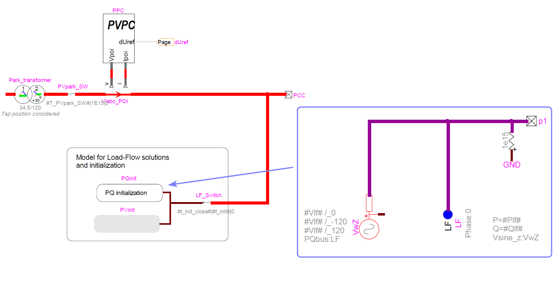
The schematic that ties this together has a few recognisable parts: the park controller — the plant-level controller EMTP® labels PVPC (a generic block name; it is the same wind-park controller, WPC, described on the architecture page) — setting the reactive/voltage reference; the park transformer feeding the point of interconnection (POI); and, off to the side, a small “model for load-flow solutions and initialisation” containing the PQ-initialisation block and the load-flow-constrained source. Two switches, the PVpark switch (the EMTP® block name for the switch to the detailed park model — the “PV” is a generic label, not a solar-PV reference) and the LF switch, decide which of these is connected at any moment.

EMTP load-flow and initialisation schematic: the external grid and park transformer at the point of interconnection, the PVpark and LF switches, and the model for load-flow solutions and initialisation containing the PQ-initialisation block and the load-flow-constrained source, feeding the detailed DFIG wind-park model.
Figure 1 — The EMTP® load-flow and initialisation arrangement for a DFIG wind park: the external grid and park transformer meet at the POI; the PVpark and LF switches select between the detailed park model and the load-flow / initialisation model, which contains the PQ-initialisation block and the load-flow-constrained source; the park controller sets the reactive/voltage reference. The switch sequence through the three phases is given in Table 1.

Section 5

The two switches that isolate the PQ source

The switches are the heart of the scheme. During the load-flow solution the PVpark switch is open and the LF switch is closed. That single arrangement means the PQ injection is connected directly to the grid and not to the internal model. Power flows from the PQ bus to the grid — not from the PQ bus, through the internal model, to the grid.

The reason is simple: during load flow the internal detailed model does not really exist — it has been removed, and only the network equations are being solved. EMTP® therefore deliberately isolates the PQ source from the detailed model. If the PVpark switch were closed during the load flow, the PQ injection would interact with an internal model that is incomplete and un-initialised, power could circulate incorrectly inside the park, and the load-flow result would be wrong. Opening the switch keeps the steady-state solve clean.

Why “all the power goes to the grid”

With the PVpark switch open, the PQ injection has only one path: to the grid. The internal model is disconnected, so no power is lost or left circulating inside the park — which is exactly the clean condition a load-flow solver needs.

Section 6

The handover: from load flow to EMT

Once the load flow has been solved, EMTP® knows the voltage magnitude and angle at every bus, the currents and the power flows. That is the operating point. The detailed model, however, is still switched out — so the transition to EMT is done in four deliberate steps.

  1. Solve the load flow. Using the PQ equivalent, obtain the steady-state voltages, angles, currents and powers.
  2. Connect the real model. Close the PVpark switch so the actual turbine, converter and controls are now in circuit — but the LF-constrained source is still holding the system.
  3. Stabilise (typically ≈0.2 s in this model). The converter finds its correct currents, the dc-link voltage settles, the machine flux and the rotor-speed / shaft states reach equilibrium, and the control loops align — all while the source pins the operating point.
  4. Release. Open the LF switch. Only the real physical model remains, and the simulation becomes a true EMT run.
Table 1 — The switch-state reference for the load-flow-to-EMT handover: for each phase, the two switch positions, whether the detailed model is connected, what holds the operating point, and whether that phase’s results should be trusted.
PhasePVpark SwitchLF SwitchDetailed Internal ModelOperating Point Held byResults to Trust?
Load-flow solutionOpenClosedRemoved — replaced by PQ injectionPQ injection, straight to the gridLoad-flow result only (no dynamics)
Initialisation (first ≈0.2 s of EMT)ClosedClosedConnected and initialisingLoad-flow-constrained sourceNo — scaffolding, not a study result
Full EMT (after release)ClosedOpenFully activeThe physical model itselfYes — assess results only here

Read top to bottom, the table tells the whole story: the PQ injection solves the point, the source then holds it while the hardware settles, and finally the physical model is left to stand on its own.

Section 7

Why the LF switch stays closed for about 0.2 s

The short window in which both switches are closed is the crucial detail. The detailed model — converter plus control — needs a little time to initialise its internal states, stabilise its control loops, and align its currents, voltages and dc-link level with the operating point. Connect it instantly, with no such window, and the result is a burst of artificial transients, an unstable start-up, and wrong results.

So EMTP® keeps the load-flow source connected while the real model is brought in. For typically around 0.2 s in this generic model (the value shown here), the source quietly enforces the correct voltage and power while the converter integrators charge, the dc-link settles and the loops lock on. That figure is not sacred: the required window depends on the controller bandwidths, the phase-locked loop (PLL) behaviour, the filter time constants, the dc-link settling time and the specific OEM / generic-model settings. The reliable rule is a condition rather than a fixed time — release the source only once the monitored variables have actually settled, and apply the studied disturbance only after that.

Avoid these
  • Energising the detailed model with no initialisation window — the run opens with artificial transients.
  • Closing the PVpark switch during the load-flow solve — the PQ source interacts with an un-initialised model and the load flow is wrong.
  • Releasing the LF switch too early, before the dc-link and control loops have settled.
  • Using the initialisation-window waveforms as results — they must not be read for fault, control-response, power-quality or stability assessment; only post-release results should be assessed.
  • Applying the studied disturbance before the source is released and the monitored variables have settled.

Section 8

What the load-flow source really is

It is tempting to picture the load-flow source as a generator or some auxiliary supply. It is neither: it is essentially a voltage source operating under a PQ constraint. In this EMTP® implementation it imposes both the terminal voltage magnitude and angle taken from the load-flow solution and the active/reactive power exchange at the connection point, so that during initialisation the rest of the model is pulled toward exactly the solved operating point. It is not a physical device — it is a numerical anchor that exists only to seed the simulation.

That distinction is the whole point when interpreting results: nothing the source does during the initialisation window is physical — it is scaffolding, not a real generator or auxiliary supply. Once it is removed (the LF switch opens), the model must hold its own operating point using only the real turbine, converter and controls, which it can because by then every internal state has been brought into agreement.

Section 9

Why EMTP® load flow is different: unbalanced and phase-by-phase

There is a second reason the load-flow capability is valuable, quite apart from initialisation. Many conventional transmission load-flow workflows use a balanced positive-sequence representation, whereas EMTP® can solve the network phase by phase. Its load flow can therefore be fully unbalanced, representing asymmetry, detailed topology and unequal phase loading that a balanced solve cannot see.

Unbalanced load flow matters in practice when the starting operating point is genuinely asymmetric — for example with collector-feeder asymmetry, particular transformer connections, single-phase loads, untransposed lines, or phase-specific faults. This is why some organisations use EMTP® purely as a load-flow engine, with no transient study in sight; for a wind park, where collector feeders and transformer connections can introduce real imbalance, the phase-by-phase solution is a meaningful advantage.

Two uses, one solver

The same load-flow capability both seeds the EMT initialisation and serves as a standalone unbalanced load-flow tool — a phase-by-phase solution most classical tools cannot provide.

Section 10

Why a consistent start matters

To see why all of this machinery is worth it, picture the converter at \(t=0\) with no initialisation. Its currents are unknown, the dc-link voltage is unknown, the controller integrators sit at zero, the machine flux is wrong and the rotor speed and shaft states are unset. The model is internally inconsistent — every state disagrees with every other — and the simulation must spend its opening instants thrashing toward equilibrium. Those instants are pure artefact, they can take a long time to settle, and they can mask or distort the very event you are trying to study.

The load-flow-plus-source scheme removes the problem at the root. The load flow supplies a physically consistent operating point; the source imposes it on the detailed model; the short window lets the controls lock onto it; and only then is the model set free. The single most important idea is that the detailed model is handed a ready-made, internally consistent operating point — its currents, dc-link voltage, fluxes, shaft states and controller integrators all in agreement — and only enters full dynamics once it demonstrably holds that point on its own.

What “consistent” means here

A clean start means every internal state agrees: the terminal voltages and currents, the dc-link voltage, the machine fluxes, the rotor-speed / shaft states and the controller integrators are all set from the same solved operating point — which is exactly what the load-flow-constrained source enforces during the initialisation window.

Section 11

Practical checks before trusting a run

A short routine confirms the initialisation has done its job:

  • Solve the load flow first and sanity-check the POI voltage, angle, \(P\) and \(Q\) against expectation; confirm the \(P/Q\) mismatch at the connection point is negligible.
  • Confirm the switch timing: PVpark open / LF closed for the solve, both closed through the initialisation window, then LF open for the run.
  • Run with no disturbance and confirm stability after release — the POI voltage, \(P\) and \(Q\), converter currents, dc-link voltage, rotor speed / torque and controller outputs should all stay flat once the LF source is released, proving the model holds the point on its own.
  • Check the dc-link voltage and control integrators have settled — and that no controller is saturating — before the LF switch opens.
  • Read only post-release results: discard the initialisation window, and apply the studied disturbance only after the source is released.
  • Where imbalance matters, exploit the unbalanced load flow rather than forcing a balanced equivalent.

Section 12

Key points

Start from a solved point, not from zero

The load-flow model gives the operating point; the switch arrangement isolates the PQ source during the solve; the load-flow-constrained source holds the point through the initialisation window; and after release, only the detailed DFIG model should define the EMT response. That is the whole scheme in one line — the EMT run begins from a consistent, solved operating point, never from zero.

References

References

  1. EMTP® Documentation and Application Notes. Powersys / EMTP®.
Built on EMTP® · Expert spotlight
Portrait of Henry Gras, Chief Operating Officer of PGSTech

Henry Gras

Chief Operating Officer, PGSTech · Montréal, Canada

Henry Gras delivers the EMTP® University course “EMT Simulation and Analysis of Large-Scale Power Systems with Renewables” and works daily with the tool this article is written around.

Henry is based in Montréal, where he is Chief Operating Officer of PGSTech, the company responsible for EMTP® engineering services, commercialisation and continuing software development. He holds a master’s degree from Polytechnique Montréal, where he worked on electrical-machine research, and previously completed an engineering degree at École Centrale de Lyon in France.

Readers who want a structured programme on EMT simulation of large-scale power systems with renewables will find his EMTP® University course an excellent next step.

Henry’s technical expertise covers electromagnetic transient simulation, renewable-energy integration, power-system modelling, electrical machines, protection and specialist transient studies including TRV, transformer energisation, ferroresonance, insulation coordination and power quality.

Thirty-Part Technical Series

EMTP® Renewable Energy Modelling

A thirty-part guide to modelling wind, PV and full-converter plant in EMTP® — sources and turbines, converter and plant control, sequence control under faults, protection, and weak-grid and SSCI stability.

Part 2 Reading now

DFIG Wind Park Load Flow and Initialisation

From a PQ equivalent to a fully initialised EMT model, with no artificial start-up transient.

Series progress 2 of 30