Renewable Modelling · AVM Principles

AVM Principles in EMTP®

Controlled AC voltage sources, DC current source and averaged power balance

An average-value converter model replaces the switching bridge with controlled sources that reproduce the converter’s averaged AC/DC power exchange. The AC side is represented by three controlled voltage sources, one per phase; the DC side is represented by a controlled current source calculated from the AC-side power. It is not just three ideal voltage sources: the phase voltages come straight from the dc-link voltage and the modulation signals, while the dc current is rebuilt from the phase currents and the same modulation signals, so the averaged AC and DC powers stay consistent within the ideal lossless model. The construction below covers where the factor of one half comes from, why the DC current source is essential for power balance, what a basic AVM leaves out, and why the converter control still acts on top of it.

Reading time ≈ 16 min · controlled sources, modulation & power balance

An average-value model is not simply three ideal voltage sources standing in for the converter. It is three controlled AC-side voltage sources and a DC-side current source, tied together so that the averaged power conversion between AC and DC stays consistent within the ideal lossless model. The DC-side current source is essential: it enforces power consistency between the AC and DC sides, so that removing the switches does not lose track of the energy drawn from or delivered to the dc link. For the higher-level comparison of the detailed and average-value models, see the detailed-versus-average-value guide.

Abbreviations used on this page

AVMAverage-value model

DMDetailed model (explicit switching)

VSCVoltage-source converter

PWMPulse-width modulation

\(m_{abc}\)Per-phase modulation signals

\(V_{dc}\)dc-link voltage

\(I_{dc}\)dc-side current (the controlled source)

\(v_{ref}\)Converter voltage reference

\(P_{ac},P_{dc}\)AC-side and dc-side power

FRTFault ride-through

EMTElectromagnetic transient

EMTP®Electromagnetic Transients Program

Key idea

An AVM replaces the converter with controlled AC-side voltage sources and a DC-side current source. The voltage sources impose the averaged terminal voltage; the current source carries the matching dc demand — so power still flows correctly between AC and DC, without explicit switching.
The AC voltages come straight from the dc-link voltage and the modulation signals, \(v_{abc}=\tfrac{1}{2}V_{dc}\,m_{abc}\); the dc current is rebuilt from the phase currents and the same modulation, \(I_{dc}=\tfrac{1}{2}(m_a i_a+m_b i_b+m_c i_c)\).
Those two together conserve power exactly: \(P_{ac}=\sum v_k i_k = V_{dc}I_{dc}=P_{dc}\). That power-balance link is the real heart of the AVM — the reason it is far more than three ideal sources.
A basic AVM is fundamental-frequency and idealised: it drops switching harmonics, semiconductor detail and losses (harmonics can be added back with switching functions). But the full converter control still acts on top of it, so it stays faithful to the controller’s intended behaviour.

Key terms used on this page

01Average-value model

A converter model built from controlled AC voltage sources and a DC current source, with no explicit switching.

02Modulation signal

The normalised per-phase command \(m\) derived from the voltage reference; \(|m|\le 1\) in the linear region.

03Controlled voltage source

An AC-side source set to the averaged phase voltage the converter would produce.

04DC current source

The dc-side source that draws the current matching the AC power, keeping the energy link consistent.

05Power balance

The condition \(P_{ac}=P_{dc}\) that the controlled-source pair enforces by construction.

06Two-level leg

A converter phase leg that connects the phase to the \(+\) or \(-\) dc rail; averaging it gives the half factor.

07Switching function

An added representation of the switching pattern that can reintroduce harmonics into an AVM.

08Fundamental frequency

The grid-frequency component a basic AVM keeps, having averaged away the switching content.

09Idealised converter

A model with no conduction, switching or dead-time losses; power conversion is loss-free.

10dc link

The dc bus the current source feeds, between the two converters of a back-to-back stage.

11Bidirectional conversion

Power can flow either way; \(I_{dc}\) changes sign as the AC power reverses.

12Control-faithful

The AVM reproduces the controller’s intended converter behaviour, omitting only the switching detail.

Section 1

From “what AVM is” to “how it is built”

It is one thing to say the AVM is simpler and faster; it is another to see how it is actually assembled. In the detailed model the IGBTs switch, the PWM creates the pattern, and the AC voltage is synthesised pulse by pulse from the switching states. The AVM skips that process entirely and imposes the averaged AC terminal voltage the converter would ideally produce. The instruction, in effect, is: do not simulate how the converter builds the voltage; just apply the averaged result — and then add a dc-side current source so the energy still balances.

DM versus AVM, in one line

The detailed model answers “how does the converter produce the voltage?”; the average-value model answers “what averaged voltage does it produce?” — with a dc current source making sure the averaged power transfer stays correct.

Section 2

Controlled sources, not switches

The core construction is short to state. On the AC side, the converter is represented by three controlled voltage sources, one per phase, set to the averaged voltage the converter would produce. On the dc side, it is represented by a single controlled current source. The voltage sources fix what the AC network sees; the current source fixes what the dc link sees. Replace the converter with only the voltage sources and you would have no proper energy link back to the dc side — so the AVM is really “replace the switching bridge by an averaged AC/DC power-conversion relation”, not merely “replace the converter by voltage sources”.

Section 3

From the voltage reference to the modulation signals

The controller still produces a voltage reference per phase, \(v_{ref,a}\), \(v_{ref,b}\), \(v_{ref,c}\), exactly as in the detailed model. In the AVM these are converted into per-phase modulation signals \(m_a\), \(m_b\), \(m_c\) — essentially the normalised control commands for each phase. Where the detailed model would feed those commands through PWM to drive the IGBTs, the AVM uses the modulation signals directly to define the averaged phase voltages. The chain shortens from “reference → PWM → gate pulses → switched voltage” to “reference → modulation signal → averaged voltage”.

Section 4

The AC-side voltage sources

Each averaged phase voltage is set directly from the dc-link voltage and that phase’s modulation signal:

\[ v_a = \tfrac{1}{2}V_{dc}\,m_a, \qquad v_b = \tfrac{1}{2}V_{dc}\,m_b, \qquad v_c = \tfrac{1}{2}V_{dc}\,m_c \]

\(v_{a},v_{b},v_{c}\): averaged converter phase voltages (relative to the dc-link mid-point)
\(V_{dc}\): dc-link voltage
\(m_a,m_b,m_c\): per-phase modulation signals, \(|m|\le 1\) in the linear region

The factor of one half is the averaged two-level leg: each phase leg connects its node to the positive or negative dc rail, and averaging that switching over a modulation interval leaves a phase voltage proportional to \(V_{dc}\) and \(m\). The scaling between dc bus, modulation command and AC voltage is physical, not arbitrary.

Section 5

The DC-side current source

This is the part that is easy to miss, and it is the real subject of this page. A converter is an energy-conversion device: if AC power is flowing out, the dc side must supply the corresponding current. Without the dc-side current source the model would impose the AC voltage but would not correctly account for the energy drawn from or delivered to the dc link — it would be a voltage source, not a converter. So the AVM includes a controlled dc current source, built from the AC phase currents and the same modulation signals:

\[ I_{dc} = \tfrac{1}{2}\big(m_a i_a + m_b i_b + m_c i_c\big) \]

\(I_{dc}\): dc-side current imposed by the controlled current source
\(i_a,i_b,i_c\): AC phase currents flowing through the converter
\(m_a,m_b,m_c\): the same per-phase modulation signals used for the voltages

The dc current is reconstructed so the dc side “feels” the power the converter processes. If the AC side delivers more power, \(I_{dc}\) changes accordingly; if the AC power reverses, \(I_{dc}\) changes sign — so the AVM still behaves as a bidirectional power converter, just without explicit switching.

Section 6

Power balance ties it all together

The two definitions are not independent — they are chosen precisely so the averaged AC and dc powers match. The dc-side current is set so that the averaged power on the AC side equals the power exchanged with the DC link, neglecting losses in the ideal AVM. Substituting the AC voltages into the AC power gives the dc power exactly:

\[ P_{ac} = v_a i_a + v_b i_b + v_c i_c = \tfrac{1}{2}V_{dc}\big(m_a i_a + m_b i_b + m_c i_c\big) = V_{dc}\,I_{dc} = P_{dc} \]

\(P_{ac}\): averaged power leaving the AC terminals
\(P_{dc}\): power drawn from the dc link

Because \(v_k=\tfrac{1}{2}V_{dc}m_k\), the AC power collapses to \(V_{dc}I_{dc}\) with the very \(I_{dc}\) defined above. Within this ideal, lossless averaged model the converter conserves power by construction — which is exactly why the model needs the DC current source and not just the AC voltage sources. A real converter has conduction, switching and dead-time losses, so the balance is exact only for the idealised AVM.

Section 7

Reading the AVM block diagram

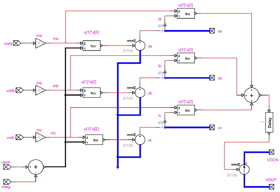
The implementation is a direct block-level realisation of those equations. On the AC side, three controlled phase-voltage sources \(v_a\), \(v_b\), \(v_c\) are built from \(V_{dc}\) and the modulation signals \(m_a\), \(m_b\), \(m_c\). On the dc side, a current source is assembled from the phase currents and the modulation signals so the dc rails see the proper current demand, with a small delay block to keep the algebraic loop well behaved. The whole averaged converter — AC voltage synthesis and dc power balance — sits in one block.

AVM principles block diagram in EMTP: the phase references vref,abc scaled by the modulation gains to ma, mb, mc; three controlled AC-side voltage sources va, vb, vc formed from the dc voltage and the modulation signals; and the phase currents combined with the modulation and summed through a delay block into the dc-side current source feeding the VDCP and VDCN rails. — Figure 1 — The AVM principles block: three controlled AC-side voltage sources set from \(V_{dc}\) and the modulation signals, and a DC-side current source built from the phase currents and modulation, realising \(v_{abc}=\tfrac{1}{2}V_{dc}m_{abc}\) and \(I_{dc}=\tfrac{1}{2}\sum_k m_k i_k\) in one averaged converter.

Section 8

What a basic AVM leaves out

Basic AVM here means the standard lossless, fundamental-frequency averaged representation, without explicit PWM switching — not every AVM variant omits every harmonic or loss mechanism. The advantage of this construction is speed: with no switching to resolve, the calculation is far faster. The price is detail. Because the model is fundamental-frequency and idealised, a few things are deliberately absent, and it is worth being explicit about what is kept and what is dropped:

Table 1 — What a basic average-value model keeps and what it omits.
Kept (Represented)	Omitted (Idealised Away)
Fundamental AC voltage and current	Switching-frequency ripple and PWM harmonics
Averaged AC/DC power transfer	Pulse-by-pulse semiconductor switching
DC-link dynamics	Dead-time effects
Controller response	Nonlinear device voltage drops
Plant–grid interaction	Conduction, switching and detailed losses

Because harmonics in a real converter come largely from the switching process, removing PWM and the IGBTs removes the switching-frequency ripple and its current harmonics, leaving the fundamental averaged behaviour. And because the converter is idealised, conduction and switching losses are not represented, so a basic AVM may slightly overestimate efficiency — acceptable for most control and system studies, but worth remembering.

Section 9

Adding harmonics back with switching functions

“Fundamental only” is the default, not a hard limit. The harmonic content a basic AVM omits can be partly reintroduced through switching functions — an added representation of the switching pattern layered onto the averaged model, so that the dominant switching-frequency components reappear without returning to a full pulse-by-pulse simulation. This is an approximation, not a replacement: switching functions can restore selected spectral content, but they do not give the full pulse-by-pulse semiconductor behaviour of a detailed model. When only specific harmonic effects matter, this can be enough; when the switching process itself is the object of study, it is not.

Section 10

The converter control still acts

This is the point that makes the AVM so useful. Removing the IGBTs and the PWM does not remove the controller. The dq current references still exist, the PI loops still run, and the voltage-reference generation, the dc-link control, the reactive-power control, the current limits and the FRT logic all remain in place — and all of them still shape the network response. The AVM still represents the controller’s intended converter behaviour; it simply skips the high-frequency switching implementation that turns that intent into pulses. That is why, for EMT studies focused on control and network interaction, the AVM gives almost everything that matters: it keeps the PLL, the loops and the plant-level dynamics while shedding only the switching detail.

Section 11

When a basic AVM is not enough

The construction makes the limits clear: an AVM is a system and control model, not a switching-harmonic model. When the switching process itself is the phenomenon of interest, the averaged converter is the wrong tool — the full detailed-versus-average-value trade-off is set out on the previous page, so here it is enough to note where the averaged converter falls short:

Where the averaged converter falls short

Switching-frequency harmonics and PWM distortion — averaged away unless switching functions are added.
Converter-side filter design and validation at high frequency — needs the real switched spectrum.
Detailed dc-side switching stress and some very fast semiconductor interactions — not represented.
Converter loss and efficiency studies — the idealised model carries no conduction or switching losses.

For those, reach for the detailed model; for control, FRT, dc-link, weak-grid and large-system studies — on a full-scale converter or a white-box generic model — the AVM remains the efficient, faithful choice.

Section 12

Key points

Controlled sources, joined by power balance

AVM replaces switching with controlled sources. Three controlled AC-side voltage sources and a DC-side current source stand in for the switching bridge, with no explicit PWM.
AC voltage is set by modulation and dc-link voltage. Each averaged phase voltage is imposed as \(v_{abc}=\tfrac{1}{2}V_{dc}m_{abc}\), the half coming from averaging the two-level leg.
The DC current source enforces power balance. \(I_{dc}=\tfrac{1}{2}(m_a i_a+m_b i_b+m_c i_c)\) makes \(P_{ac}=V_{dc}I_{dc}=P_{dc}\) within the ideal lossless model — the reason the model is more than three voltage sources.
A basic AVM omits switching ripple and losses. It is fundamental-frequency and idealised; switching functions can add selected harmonics back.
The converter control still acts — dq loops, dc-link, reactive-power and FRT all remain — which is why the AVM is the efficient, faithful choice for large control and system EMT studies, unless the switching process itself is the subject (then use the detailed model).

References

EMTP® Documentation and Application Notes. Powersys / EMTP®.

Built on EMTP® · Expert spotlight

Henry Gras

Chief Operating Officer, PGSTech · Montréal, Canada

Henry Gras delivers the EMTP® University course “EMT Simulation and Analysis of Large-Scale Power Systems with Renewables” and works daily with the tool this article is written around.

Henry is based in Montréal, where he is Chief Operating Officer of PGSTech, the company responsible for EMTP® engineering services, commercialisation and continuing software development. He holds a master’s degree from Polytechnique Montréal, where he worked on electrical-machine research, and previously completed an engineering degree at École Centrale de Lyon in France.

Readers who want a structured programme on EMT simulation of large-scale power systems with renewables will find his EMTP® University course an excellent next step.

Henry’s technical expertise covers electromagnetic transient simulation, renewable-energy integration, power-system modelling, electrical machines, protection and specialist transient studies including TRV, transformer energisation, ferroresonance, insulation coordination and power quality.

Part 19 Reading now

AVM Principles: the Controlled-Source Model

Building the average-value converter from controlled sources that reproduce the fundamental behaviour without switching.

Series progress 19 of 30

Part 20

Protection in Renewable EMT Models

Voltage relays, deep-sag blocking, the dc chopper and device protection in renewable EMT models.