Renewable Modelling · Impedance-Scan SSCI Screening

Time-Domain Impedance Scanning for SSCI in EMTP®

Combining grid and turbine impedance for SSCI screening

SSCI risk depends on the interaction between the frequency-dependent grid impedance and the active impedance of the turbine converter. A time-domain impedance scan is a practical way to screen many operating conditions before running detailed EMT validation cases. Split the network at the turbine terminal; represent the external grid by its frequency-dependent impedance and the converter-plus-filters by theirs (the turbine side extracted by a time-domain perturbation scan, because converters are nonlinear and full of control loops); combine them; and flag any frequency where the total reactance crosses zero while the resistance is negative — resonance with negative damping. What follows sets out the split, why impedance is the right language, the zero-reactance / negative-resistance criterion, and why it is a screening tool that EMT then confirms.

Reading time ≈ 18 min · combined impedance scan & resonance/damping test

Sub-synchronous control interaction (SSCI) is an oscillatory interaction between converter controls and the electrical network at frequencies below the fundamental, and it depends on so many factors — wind speed, filter settings, control mode, grid strength — that testing every case in full time-domain is impractical. The impedance scan offers a way out: characterise each side as a frequency-dependent impedance, combine them, and read off where the combination looks unstable. It is a fast screen for the risky operating modes before any heavy EMT validation. This is a different question from the harmonic frequency scan: harmonic studies look at the distortion produced by injected harmonic currents, whereas SSCI impedance scanning looks at the stability of the interaction between converter control and the network impedance.

Abbreviations used on this page

SSCISub-synchronous control interaction

\(Z(f)\)Frequency-dependent impedance

\(R,X\)Resistance, reactance

\(f^{\ast}\)Frequency of concern

TDTime domain

EMTElectromagnetic transient

PLLPhase-locked loop

SCRShort-circuit ratio (grid strength)

Q/VReactive-power / voltage control mode

WTWind turbine

DFIGDoubly-fed induction generator

EMTP®Electromagnetic Transients Program

Key idea

SSCI is an interaction between converter control and grid, so the right language is impedance: how each side responds to a small disturbance at each frequency. The network is split at the turbine terminal into a grid side and a turbine side.
The turbine-side impedance is extracted by a time-domain perturbation scan (“Input Impedance TD”), because a converter is nonlinear and full of limiters, a PLL, filters and dq loops — a pure analytical derivation is rarely enough.
Combine the two sides, \(Z_{total}=Z_{grid}+Z_{turbine}\), and flag a frequency where the total reactance crosses zero (a resonance) while the total resistance is negative (negative damping) — the signature of potential instability.
Because the turbine signature changes with the operating point and control mode, the method screens many conditions fast; detailed EMT validation is then run only on the flagged cases. It is a screen, not a final proof.

Key terms used on this page

01SSCI

Sub-synchronous control interaction: an oscillatory instability between converter control and grid.

02Impedance scan

Mapping a side’s impedance versus frequency to judge how it responds to small disturbances.

03Input Impedance TD

Turbine impedance extracted from a time-domain perturbation simulation, not a pure analytical model.

04Interface point

The bus where the network is split and the two impedances are measured and combined.

05Grid-side impedance

\(Z_{grid}(f)\): the external grid, transformers and collector equivalent seen from the interface.

06Turbine-side impedance

\(Z_{turbine}(f)\): the converter, control and filters seen from the interface.

07Zero reactance

A frequency where \(X_{total}=0\); inductive and capacitive parts cancel — a resonance candidate.

08Negative resistance

\(R_{total}\) below zero: the combination feeds energy into the oscillation rather than damping it.

09Negative damping

The condition under which an oscillation grows rather than decays.

10Operating point

Wind speed, control mode, reactive output and limits — all of which reshape the turbine impedance.

11Grid strength (SCR)

How stiff the grid is; a weak grid (low SCR) raises the interaction risk.

12Screening

Quickly flagging risky conditions, to be confirmed by targeted EMT validation.

Section 1

Screening SSCI risk

The purpose of this method is screening and diagnosis. Rather than testing every operating case in full time-domain, it asks a sharper question: for this operating point, does the converter–grid combination look potentially unstable? The answer comes from impedances rather than waveforms, which is what makes it fast enough to sweep across conditions.

The question the scan answers

“For this operating point, does the converter–grid combination look potentially unstable?” — answered by combining two frequency-dependent impedances and inspecting the result, not by running a full transient for every case.

Section 2

Why brute-force EMT is painful

SSCI can depend on the wind speed, the filter settings, the operating mode, whether the plant is in reactive-power or voltage control, the grid strength and the operating point. Studying every combination with detailed time-domain simulation alone would mean many operating points, many grid strengths, many disturbances and a great deal of simulation time. The impedance scan replaces that with a fast signature for each condition, so the heavy time-domain runs can be reserved for the few cases that actually look risky.

Section 3

Splitting the network at an interface

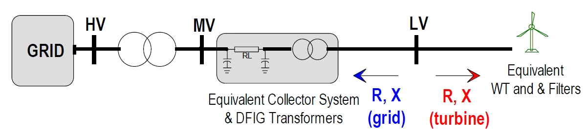
The method begins by choosing an interface point — here the turbine terminal, at the low-voltage side of the collector system — and looking both ways from it. The interface point must be selected consistently: looking outward from it gives the grid-side impedance, and looking inward gives the turbine/converter-side impedance. Looking outward is the external system: the high-voltage grid, the transformers, the medium-voltage system and the collector equivalent, gathered into \(Z_{grid}(f)\). Looking inward is the turbine, converter and filters, gathered into \(Z_{turbine}(f)\). The two sides face each other like dynamic Thévenin/Norton impedances at that common point.

Single-line diagram of the wind-turbine interface split. From left: the GRID, an HV bus and transformer, an MV bus, the equivalent collector system and DFIG transformers (an RL branch with shunt capacitances and a transformer), an LV bus, and the equivalent wind turbine and filters on the right. At the LV interface two arrows show the impedance split: R and X looking left into the grid and collector, and R and X looking right into the turbine and its filters. — Figure 1 — The interface split: \(Z_{grid}\) looking into the grid and collector, \(Z_{turbine}\) looking into the converter and filters, combined at the turbine terminal into \(Z_{total}=Z_{grid}+Z_{turbine}\).

Section 4

Why impedance is the right language

Converter instability is not simply “too much current” or “too much voltage” — it is an interaction. The turbine control has a dynamic electrical behaviour; the grid has a dynamic electrical behaviour; and at some frequencies those two behaviours can reinforce each other. So instead of asking only what the current or voltage is, the useful question is how each side responds to a small disturbance at each frequency. That response is exactly what impedance captures, which is why it is the natural language for this kind of stability problem.

Section 5

What “Input Impedance TD” means

The grid side is usually passive and linear enough to characterise with a straightforward frequency-domain scan. The turbine side is different, and the “TD” matters: its impedance — the input impedance seen looking into the converter, which is exactly \(Z_{turbine}(f)\) — is obtained from a time-domain perturbation-based analysis, not only from a classical linear frequency-domain block model. That is because a converter is active, nonlinear and controlled — full of limiters, a phase-locked loop, filters and dq current loops — so a textbook frequency-domain derivation is often not enough or not practical.

In practice a small voltage or current perturbation is injected at selected frequencies, and the measured response is used to calculate the effective impedance at each frequency; the time-domain scan extracts that impedance directly from simulation, which makes it far more realistic for converter-based systems. In a fuller treatment the converter impedance is a dq matrix with coupling between the d- and q-axes; for screening, the scalar resistance–reactance reading used here is usually enough.

Section 6

The combined scan

With both sides characterised, the combined scan adds them. Each is a complex, frequency-dependent impedance, and at the interface they sit in series, so their real and imaginary parts add:

\[ Z_{total}(f) = Z_{grid}(f) + Z_{turbine}(f) = \underbrace{\big(R_{grid}+R_{turbine}\big)}_{R_{total}(f)} + j\,\underbrace{\big(X_{grid}+X_{turbine}\big)}_{X_{total}(f)} \]

\(Z_{grid}=R_{grid}+jX_{grid}\): external grid and collector impedance at the interface
\(Z_{turbine}=R_{turbine}+jX_{turbine}\): converter, control and filter impedance at the interface
\(R_{total},X_{total}\): total resistance and reactance seen at the interface

The grid scan and the turbine scan are run separately and then summed — which is why one turbine signature can be tested against many grid cases, or many turbine signatures against one grid case, simply by re-combining.

Section 7

The instability criterion

The combined impedance is read at every frequency, looking for one signature. Where the total reactance crosses zero, the inductive and capacitive parts cancel — a resonance, a frequency at which the electrical system can naturally oscillate. But resonance alone does not make an oscillation grow; that depends on the resistance. If the total resistance at that same frequency is negative, the combination is not damping the oscillation but feeding energy into it. Negative resistance here does not mean a physical resistor is negative; it means the active converter-control response can feed energy into the oscillation instead of damping it. Together, those two conditions are the warning sign:

\[ \text{potential instability at } f^{\ast}: \qquad X_{total}(f^{\ast}) = 0 \quad \text{and} \quad R_{total}(f^{\ast}) \lt 0 \]

\(f^{\ast}\): the frequency at which the reactance crosses zero
\(X_{total}(f^{\ast})=0\): a resonance candidate (reactances cancel)
\(R_{total}(f^{\ast})\lt 0\): negative damping (energy fed into the oscillation)

Zero reactance gives a frequency where the system can oscillate; negative resistance at that frequency means the oscillation grows rather than decays. Neither alone is sufficient — it is the combination that flags potential instability. The negative resistance must also be relevant at or close to the resonance frequency: a negative resistance at some unrelated frequency, away from a zero-reactance crossing, is not by itself an SSCI problem.

Table 1 — Reading the combined impedance at each frequency.
Condition	Meaning	Verdict
\(X_{total}\ne 0\)	Reactances do not cancel	Not a resonance candidate
\(X_{total}=0\), resistance positive	Resonance with positive damping	Damped — stable
\(X_{total}=0\), resistance negative	Resonance with negative damping	Potentially unstable — flag

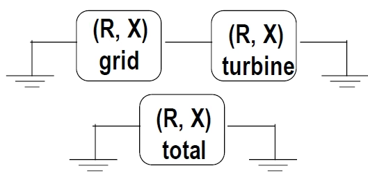
A block diagram of the impedance split: an (R, X) grid block and an (R, X) turbine block in the top row, each referenced to ground, and an (R, X) total block below, showing that the grid and turbine impedances add to the total impedance seen at the interface. — Figure 2 — Forming the total: the grid and turbine (R, X) contributions add to the total (R, X) at the interface. The instability signature is then read from that total — a frequency where \(X_{total}\) crosses zero while \(R_{total}\) is negative.

Section 8

Why it depends on the operating point

A converter is not a passive impedance like a fixed resistor or inductor; it is an active, controlled element, so its effective impedance changes with the conditions. In practice \(Z_{turbine}(f)\) changes with the wind speed and active power, the reactive-power or voltage-control mode, the PLL settings, the filters, the current limits and the controller bandwidth. So the turbine scan is really a family of signatures, not one universal curve, and the grid impedance is not fixed either:

Table 2 — What each side’s impedance depends on.
Grid impedance \(Z_{grid}\) depends on	Turbine impedance \(Z_{turbine}\) depends on
Network topology and connections	Control mode (reactive-power or voltage)
Transformer and cable status	Wind speed and operating point
Shunt devices	Reactive power being generated
System strength (short-circuit ratio)	PLL state and tuning
Other plant conditions	Current limits and filter settings

Section 9

The grid changes too

Because the grid impedance varies with topology, transformer and cable status, shunt devices, system strength and the state of other plant, the same plant can be stable against one grid configuration and risky against another. That is exactly what makes the combined-scan method powerful for sensitivity analysis: you can test one turbine signature against many grid cases, or many turbine signatures against one grid case, simply by re-summing the scans — covering a wide envelope of conditions without a full transient for each.

Section 10

A screening tool, not a final proof

It is worth being precise about what the method delivers: it detects potentially unstable operating modes. A zero-crossing with negative resistance does not guarantee catastrophic instability in every full simulation, nor that no other mechanism matters. What it does is tell you where the risky zones are. Once a risky operating point is found, the usual next step is detailed EMT time-domain validation — perhaps a specific fault or switching event, perhaps controller retuning. So the impedance scan is a screening and interpretation tool, and EMT confirms. The concrete output is a list of the operating conditions and frequencies at which the combined impedance shows a resonance with poor or negative damping, together with the selected EMT validation cases that follow — and those EMT runs confirm whether the oscillation actually grows under realistic controls, limits and disturbances.

Screen, then confirm

The scan flags the suspicious conditions cheaply; the targeted EMT run confirms (or clears) them. The value is in not having to run the heavy study for every combination — only for the ones the scan marks.

Section 11

The study workflow

Put together, the combined-scan workflow is six steps:

Extract the grid-side impedance scan \(Z_{grid}(f)\).
Extract the turbine-side impedance scan \(Z_{turbine}(f)\) for the operating condition, by time-domain perturbation.
Combine them: \(Z_{total}(f)=Z_{grid}(f)+Z_{turbine}(f)\).
Find the frequencies where \(X_{total}(f)=0\), and check whether \(R_{total}(f)\) is negative there.
Flag those operating conditions as potentially unstable.
Validate only the flagged cases with targeted EMT time-domain runs.

Section 12

Key points

Resonance plus negative damping, found by combining impedances

SSCI depends on the interaction between the grid impedance and the converter impedance, so impedance is the right language for screening it.
The system is split at a defined interface (the turbine terminal) into a grid side \(Z_{grid}(f)\) and a turbine side \(Z_{turbine}(f)\), the latter extracted by a time-domain perturbation scan.
The turbine impedance is operating-point dependent — it changes with wind speed, control mode, PLL, filters, current limits and controller bandwidth — so it is a family of signatures.
A potentially unstable condition is flagged where the total reactance crosses zero and the resistance is negative at that frequency (resonance with negative damping).
EMT validation is still required for the flagged cases: the scan screens, and a targeted EMT run confirms whether the oscillation actually grows.

For the related studies, see the harmonic frequency-scan, SSCI parameter and wind-park modelling guides.

References

EMTP® Documentation and Application Notes. Powersys / EMTP®.

Built on EMTP® · Expert spotlight

Henry Gras

Chief Operating Officer, PGSTech · Montréal, Canada

Henry Gras delivers the EMTP® University course “EMT Simulation and Analysis of Large-Scale Power Systems with Renewables” and works daily with the tool this article is written around.

Henry is based in Montréal, where he is Chief Operating Officer of PGSTech, the company responsible for EMTP® engineering services, commercialisation and continuing software development. He holds a master’s degree from Polytechnique Montréal, where he worked on electrical-machine research, and previously completed an engineering degree at École Centrale de Lyon in France.

Readers who want a structured programme on EMT simulation of large-scale power systems with renewables will find his EMTP® University course an excellent next step.

Henry’s technical expertise covers electromagnetic transient simulation, renewable-energy integration, power-system modelling, electrical machines, protection and specialist transient studies including TRV, transformer energisation, ferroresonance, insulation coordination and power quality.

Part 26 Reading now

Time-Domain Impedance Scanning for SSCI

Time-domain impedance scanning that combines the grid and turbine impedance for SSCI screening.

Series progress 26 of 30

Part 27

The Grid-Side Impedance Scan for SSCI

The grid-side scan under series compensation and post-fault topology, and reading R(f) and X(f).