Lightning Transients · Waveform Selection

Lightning Current and Switching Surge Waveforms for Transient Studies

The waveform used in a lightning or switching transient study is not a cosmetic input. It can strongly influence the calculated tower voltage, footing response, surge-arrester duty, incoming surge shape, insulation stress, travelling-wave reflections and electromagnetic coupling. The waveform should be chosen from the physical phenomenon being represented — first stroke, subsequent stroke or switching surge — and the study objective, not from whichever mathematical shape is easiest to enter. This guide sets out the standard impulse definitions, why the maximum steepness matters as much as the peak, and how the triangular, double-exponential, CIGRE-concave, Heidler and double-peaked representations differ in practice.

Reading time ≈ 26 min · Lightning & switching waveform guide

In a practical EMTP® or insulation-coordination study the engineer normally has to define the current or voltage peak, the front time (time-to-crest), the maximum steepness, the tail (time-to-half), the polarity, whether the event is a first stroke, a subsequent stroke or a switching surge, and whether the waveform is for simplified screening or detailed transient modelling. The key point is that different studies need different waveforms: a simple triangular shape can be acceptable for screening; a CIGRE-concave or double-peaked shape is better for first-stroke lightning-performance work; a Heidler function suits cases needing a smooth differentiable curve; and a switching impulse lives on a completely different time scale and must not be treated like a lightning impulse.

Abbreviations used on this page

EMTP®Electromagnetic Transients Program

\(I_P\)Peak current

\(t_f\)Lightning front time (virtual, from the 30–90% points)

\(T_p\)Switching time-to-crest (actual time-to-peak; sometimes written \(t_c\))

\(t_h\)Time-to-half value (tail)

\(S_m\)Maximum current steepness, \(\max(dI/dt)\)

\(R_E\)Tower-footing / electrode resistance

\(L_T\)Equivalent tower inductance

FFO / SFOFast-front / slow-front overvoltage

Key idea

The waveform sets the frequency content and severity of the transient — match it to the stroke type and study objective, not to mathematical convenience.
For first strokes the maximum steepness sits near the first peak. Triangular, CIGRE-concave and double-peaked shapes can place it there; a double-exponential puts its maximum rate of rise at the start, so it can misrepresent front stress.
Preserve the parameters that control the result: peak current, front time, maximum steepness, time-to-half and, where relevant, the second peak.
Switching surges are produced by the network event (breaker timing, trapped charge, line length, compensation), not imposed as a 250/2500 µs source — that notation is for withstand comparison.

Key terms used on this page

01Front time \(t_f\)

The time characterising the rising edge; for a lightning impulse voltage a virtual front time derived from the 30% and 90% points.

02Time-to-half \(t_h\)

Time from the (virtual) origin to the point on the tail where the wave has fallen to 50% of crest.

03Maximum steepness \(S_m\)

The largest value of \(dI/dt\) on the front, in kA/µs; drives the inductive part of tower and footing voltage.

04First return stroke

Usually the highest-amplitude stroke; concave front, steep rise to a first peak, often a higher second peak.

05Subsequent stroke

Lower peak but much shorter, steeper front; important for fast-front and high-frequency effects.

06Double-exponential

\(i(t)=I_0(e^{-\alpha t}-e^{-\beta t})\); smooth and simple, but its maximum steepness is at the start.

07Heidler function

A smooth, continuously differentiable lightning-current function; combinable to build realistic shapes.

08CIGRE-concave

A waveform with separate front and tail expressions that reproduces the concave front of measured first strokes.

09Double-peaked

A first/second-peak shape, typically a sum of Heidler functions fitted to measured parameters.

10Triangular / ramp

A linear rise to peak then an assumed tail; simple, defined by an average front steepness.

11Lightning impulse (1.2/50)

Standard test voltage: \(\approx\)1.2 µs front, 50 µs time-to-half — a withstand reference, not a stroke current.

12Switching impulse (250/2500)

Standard slow-front test waveform: 250 µs to crest, 2500 µs time-to-half.

Section 1

Why the waveform is a physical input, not a formality

The shape of the injected wave decides which frequencies the network is excited at, and therefore how severe the response is. A fast front rich in high-frequency content stresses tower surge response, footing transient impedance, travelling-wave reflections and arrester duty; a slow front does not. Two waves with the same peak can give different answers if their fronts differ. So before choosing a waveform, decide what physical event is being represented and which output parameter controls the result — then pick a shape that preserves that parameter. The rest of this guide works through the standard definitions and the common analytical shapes with that principle in mind.

Section 2

Standard impulse waveform definitions

Impulse waveforms are described by two time parameters — a front time and a time-to-half value. For a standard lightning impulse voltage, the virtual front time is defined from the 30% and 90% points of the crest:

\[ t_f = 1.67\,(t_{90}-t_{30}) \]

\(t_f\): virtual front time
\(t_{30}\): actual time at 30% of crest
\(t_{90}\): actual time at 90% of crest

The factor \(1.67=1/0.6\) projects the 30–90% interval onto a virtual 0–100% front, referred to a virtual origin \(O_1\) (IEC 60060-1, the high-voltage impulse test-technique standard); the time-to-half \(t_h\) then runs from \(O_1\) to the 50% point on the tail. A standard lightning impulse voltage is written 1.2/50 µs (front 1.2 µs ±30%, half-value 50 µs ±20%). A standard switching impulse is 250/2500 µs, but its front is the actual time to peak \(T_p\) (250 µs) measured from the true origin, with the time-to-half (2500 µs) from that same origin — so the essential difference is a virtual front time (lightning) versus an actual time-to-peak (switching), not the tail reference. Lightning impulses are fast-front events; switching impulses are slow-front; they excite different frequency ranges and so need different modelling assumptions.

Section 3

Lightning current is not the standard impulse voltage

The 1.2/50 µs lightning impulse is a test voltage waveform for equipment withstand and insulation coordination. It should not be used automatically as the lightning current waveform in a system transient study. Measured lightning currents have richer shapes: a first return stroke typically shows an initial concave front, a steep near-linear rise to a first peak, maximum steepness in the upper part of the front just before crest, a second peak a few microseconds later (sometimes comparable to or higher than the first), and possible subsidiary peaks on the decay. A median or normalised double-exponential curve can be statistically convenient, but averaging removes exactly the features — concave front, first and second peaks, local steepness — that often control the result. For a transient study the current waveform should preserve peak current, maximum steepness, front time, the time of the first (and, if relevant, second) peak, and the tail duration. In an EMT study, inject a representative concave-front current source — for line studies, a median first stroke of order 30 kA with a few-microsecond front, built from a Heidler or CIGRE-concave function — not the 1.2/50 µs test voltage.

Section 4

The first return stroke

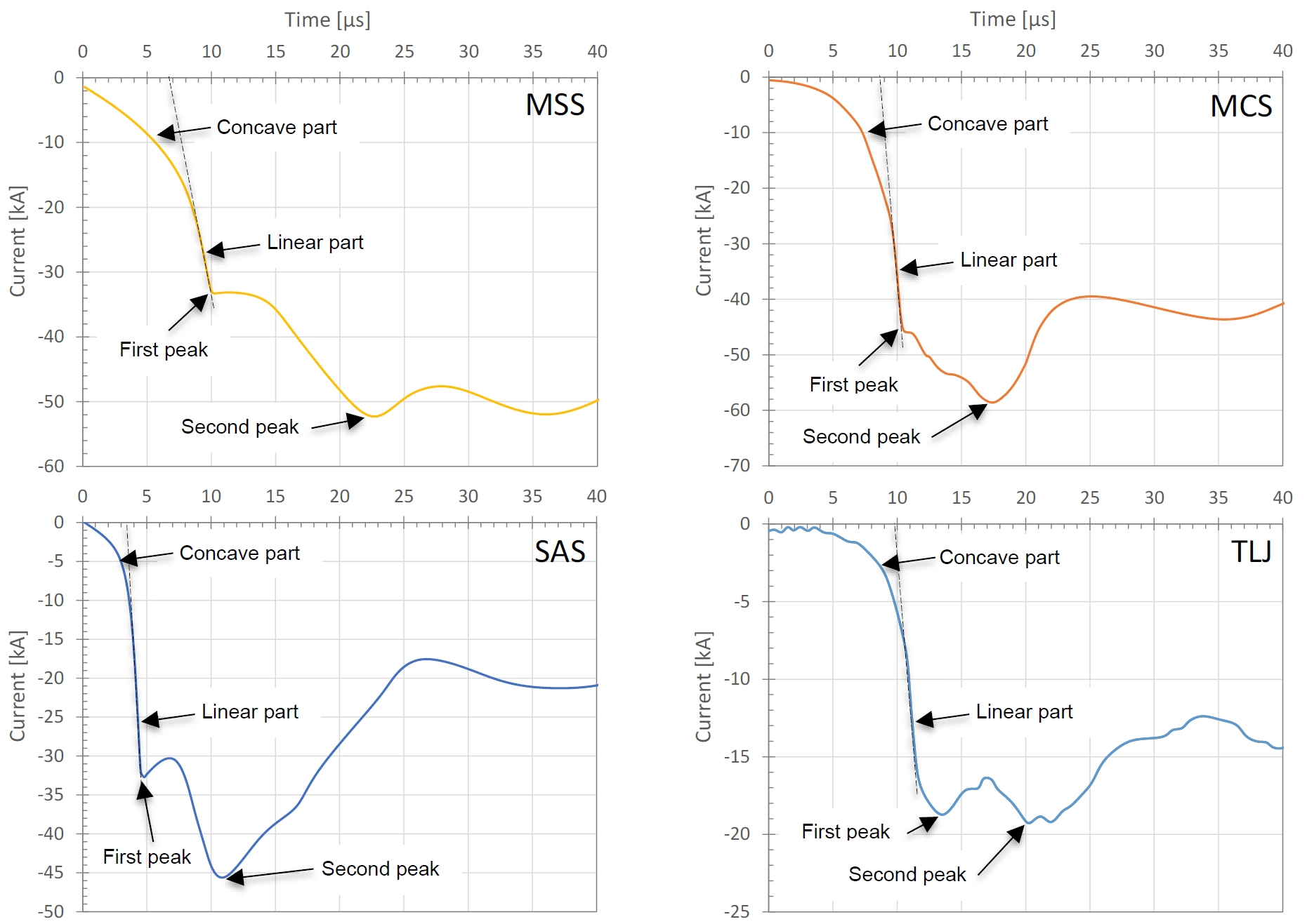
The first return stroke is normally the most important for transmission-line lightning performance, because it usually carries the highest current and is associated with backflashover, shielding failure, tower-footing voltage rise and incoming-surge calculations. A realistic first-stroke representation should capture that the front is not purely linear from the origin, the first part can be concave, the steepest part is usually just before the first peak, the first peak comes early, a second peak can follow a few microseconds later, and the tail can remain significant for tens of microseconds.

Four measured first downward negative return-stroke current waveforms (stations MSS, MCS, SAS and TLJ), each annotated with a concave part, a linear part, a first peak and a second peak; current in kA versus time in microseconds. — **Figure 1 —** Typical measured first downward negative-stroke current waveshapes from four stations — MSS (Mount San Salvatore), MCS (Morro do Cachimbo), SAS (South Africa) and TLJ (Japanese transmission lines). Each record shows a **concave front**, a steep near-linear rise to the **first peak**, and a **second peak** a few microseconds later. Real first strokes are not smooth double-exponential curves, so the waveform used in a study should preserve peak current, maximum steepness and front-time behaviour. *(Station data shown for illustration.)*

Section 5

Why maximum steepness matters

In a simplified tower model the tower-top voltage has an inductive part driven by the rate of rise of current and a resistive part driven by its magnitude:

\[ V_L = L_T\,\frac{dI(t)}{dt} \qquad\qquad V_R = I(t)\,R_E \] \[ V_{TT} \approx L_T\,\frac{dI(t)}{dt} + I(t)\,R_E \]

\(V_{TT}\): simplified tower-top voltage
\(V_L,\ V_R\): inductive and resistive contributions
\(L_T\): equivalent tower inductance
\(R_E\): tower-footing resistance — at lightning currents, the current-dependent impulse (ionised) value
\(dI/dt\): current steepness

Two cautions make this a screening estimate only. First, the terms do not peak together: \(L_T\,dI/dt\) peaks near the maximum steepness on the front, while \(I(t)R_E\) peaks at crest — so \(V_{TT}\) is not the arithmetic sum of the two maxima. Second, \(R_E\) should be the current-dependent impulse (ionised) footing resistance, not the low-current measured value, and \(L_T\) is a lumped surrogate for the tower surge impedance \(Z_T\) with travel time \(\tau=2h/c\). The expression also ignores travelling-wave reflections, conductor coupling and the footing’s transient impedance, so it is not a replacement for an EMTP® or HIFREQ model. Still, it shows why shape matters: the inductive term is set by steepness, the resistive term by magnitude, so two waveforms with the same peak but different steepness give different voltages.

The maximum steepness is defined as

\[ S_m = \max\!\left(\frac{dI}{dt}\right) \]

\(S_m\): maximum current steepness, kA/µs
\(I,\ t\): lightning current and time

For tower and overhead-line studies \(S_m\) can matter as much as peak current: a high peak with a slow front can be less onerous than a lower peak with a very steep front. Fast fronts carry higher-frequency content that affects tower surge response, shield-wire coupling, footing transient impedance, travelling-wave reflections, induced voltages and arrester duty. A first-stroke waveform should therefore place \(S_m\) close to the first peak, consistent with measurements — one reason not all analytical shapes suit backflashover work.

Section 6

Analytical waveforms for the first stroke

Several analytical waveforms are used to represent first-return-stroke currents — the triangular (ramp-slope), the double-exponential, the CIGRE-concave, single or multiple Heidler functions, and the double-peaked shape. Each has a distinct purpose and limitation, set out in the next sections.

Section 7

Triangular / ramp-slope waveform

The triangular waveform rises linearly to the peak and then decays on an assumed tail. Its advantage is simplicity, and the front steepness is explicit:

\[ S = \frac{I_P}{t_f} \]

\(S\): average front steepness
\(I_P\): peak current
\(t_f\): front time

If the ramp is set to the required maximum steepness it is useful for simplified lightning-performance calculations. The drawback is a sharp corner at the peak (unless smoothed), which can inject artificial high-frequency content into a simulation, and it reproduces neither the concave front nor the double peak. Use it for screening, simplified performance and steepness-driven sensitivity studies, or where a method specifically calls for a ramp. Avoid it when a smooth numerical waveform is needed, the second peak matters, or the aim is to reproduce a measured shape. In detailed EMTP® studies, avoid sharp discontinuities unless the numerical effect is understood and the time-step is suitable.

Section 8

Double-exponential waveform

The double-exponential has long been used because it is mathematically simple, smooth, and convenient for laboratory impulse generation:

\[ i(t)=I_0\left(e^{-\alpha t}-e^{-\beta t}\right) \]

\(i(t)\): current at time \(t\)
\(I_0\): scaling constant set to obtain the required peak
\(\alpha,\ \beta\): tail and front time constants, units \(\mu\text{s}^{-1}\) (or \(\text{s}^{-1}\)); \(\beta>\alpha\)

The actual peak is below \(I_0\) and occurs at \(t_{\text{pk}}=\dfrac{\ln(\beta/\alpha)}{\beta-\alpha}\). Its key limitation for first strokes: with \(\beta>\alpha\) the maximum rate of rise is at the beginning (\(t=0\), where \(di/dt=I_0(\beta-\alpha)\)) and then decreases toward the peak, giving an unphysical convex front — the opposite of the measured concave front whose steepest part is near the first peak. This convex-versus-concave mismatch is exactly why the smooth Heidler form superseded the double-exponential for first-stroke work. It may be acceptable for general impulse representation or laboratory waveform matching, but it should not be the default choice for first-stroke tower-voltage or backflashover studies where the timing of maximum steepness is important.

Section 9

CIGRE-concave waveform

The CIGRE-concave waveform (CIGRE — the International Council on Large Electric Systems) was developed to represent measured first return strokes more faithfully. It uses separate expressions for the wavefront and the wavetail, so the concave front and the steep rise toward the first peak can be controlled independently of the tail. That makes it more suitable than a double-exponential for lightning-performance studies where tower voltage and line-insulation stress are governed by the current front. It suits first downward negative-stroke studies, transmission-line performance, tower overvoltage and backflashover work, and any case where steepness near the first peak matters. Its only real cost is that it is more involved than a triangular or double-exponential shape — justified whenever the front shape affects the answer.

Section 10

The Heidler function

The Heidler function is widely used in EMT studies because it gives a smooth, continuously differentiable current with no discontinuity in the derivative:

\[ i(t)=\frac{I_P}{\eta}\,\frac{(t/\tau_1)^{n}}{1+(t/\tau_1)^{n}}\,e^{-t/\tau_2} \]

\(i(t)\): lightning current at time \(t\)
\(t\): time, on the same unit basis as \(\tau_1,\ \tau_2\)
\(I_P\): target peak current
\(\eta\): peak-correction factor
\(\tau_1\): front time constant (\(\mu\text{s}\) or s)
\(\tau_2\): tail time constant (\(\mu\text{s}\) or s)
\(n\): front-steepness exponent (dimensionless, typically 2–10)

The correction factor \(\eta=\exp\!\big[-(\tau_1/\tau_2)\,(n\,\tau_2/\tau_1)^{1/n}\big]\) makes the function’s actual peak equal \(I_P\). Because it is differentiable, the Heidler form is numerically stable and avoids the artificial high-frequency content of a sharp ramp. A single Heidler function cannot independently reproduce both the first and second peaks, so realistic first strokes are built by summing several. Use it when a smooth waveform is needed, the simulation is sensitive to discontinuities, or parameters must be fitted to measured/standard data.

Section 11

Double-peaked waveform

Measured first strokes often show a first peak followed by a (frequently higher) second peak. A double-peaked waveform reproduces this, most commonly by summing multiple Heidler functions so the engineer can fit first peak, second peak, front time, maximum steepness, time-to-half and overall shape together. The benefit is realism — it matches the main measured parameters of first return strokes more closely than any single analytical function. The cost is more parameters and more care in implementation, and it is not needed for simplified screening. Use it when the second peak affects the result, the study aims to reproduce measured behaviour, the timing of peak voltage and current matters, or the model feeds a detailed lightning-performance assessment.

Section 12

Which first-stroke waveform should be used?

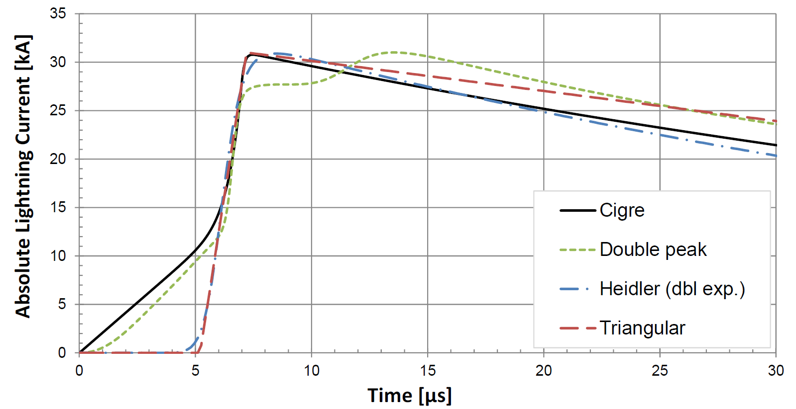
Comparison plot of four analytical first-return-stroke current waveforms — CIGRE concave, double-peak, Heidler and triangular — absolute lightning current in kA versus time in microseconds, all reaching a similar peak near 31 kA. — **Figure 2 —** Analytical representations of a first return-stroke current — CIGRE-concave, double-peak, Heidler and triangular. (The blue curve is a Heidler function — its delayed, concave front is not a true double-exponential, so the legend’s “dbl exp.” label is loose.) All reach a *similar* peak (here near 31 kA around 7 µs) yet differ in front shape, in **where the maximum steepness occurs** and in the tail. Two waveforms with the same peak current can therefore give different calculated transient voltages.

The right choice follows the study objective. For simplified line lightning-performance calculations, a triangular/ramp waveform can be acceptable where the method is based on maximum steepness and a specified front time. For more realistic first-stroke studies the CIGRE-concave waveform is generally preferable, because it represents the concave front and the steep rise near the first peak. For numerical EMT studies where smoothness matters, a Heidler-based waveform is often preferred. For detailed studies that must reproduce measured behaviour, a double-peaked (multi-Heidler) waveform represents the first peak, second peak, front time, time-to-half and maximum steepness more independently. A double-exponential should be used cautiously in first-stroke backflashover or tower-voltage work, because its maximum steepness is at the start rather than near the first peak.

Quick rule

Triangular/ramp → simplified, steepness-based methods. CIGRE-concave → practical first-stroke performance. Heidler → when a smooth analytical waveform is required. Double-peaked → when first and second peaks must both be represented. Double-exponential → avoid relying on it when the timing of maximum steepness controls the result.

Section 13

Subsequent return strokes

Subsequent strokes differ from first strokes: lower peak current but a much shorter, steeper front. The current rises quickly to a single dominant peak and decays with a shorter time-to-half. A typical subsequent stroke has a front of roughly 0.2–5 µs, a single peak, a shorter tail than a first stroke, and very high steepness. Because the front is so fast, subsequent strokes can dominate fast-front overvoltage, induced-voltage and coupling studies, surge-arrester response and high-frequency interference — they may not give the highest tower voltage from magnitude alone, but they produce severe high-frequency effects. They are usually represented by Heidler functions, which give a fast smooth front and a realistic tail without numerical discontinuities.

Representative parameters (dataset-dependent)

A subsequent-stroke waveform might use, for example, a peak current near 11.8 kA, a 30–90% front time near 0.4 µs, a maximum steepness near 39.9 kA/µs and a time-to-half near 32 µs — representative of the CIGRE TB 549 / Anderson–Eriksson subsequent-stroke distribution (peak near the ~12 kA median). These figures are consistent, not contradictory: a 0.4 µs 30–90% front gives an average slope near 17.7 kA/µs, while the 39.9 kA/µs is the maximum rate of rise near crest (about 2.3× the average), as a concave front produces — so it is not \(11.8/39.9\). The very high steepness with a modest peak is what makes subsequent strokes a fast-front concern; treat the specific numbers as illustrative and take them from the standard or dataset your study is based on.

Section 14

Switching surge waveforms

Switching transients are slow-front, long-tail voltage events — switching surge overvoltages, not an injected current. The standard switching impulse voltage is 250/2500 µs (250 µs time-to-crest, 2500 µs time-to-half) and is relevant to line energisation, reclosing, load rejection, capacitor and shunt-reactor switching, transformer energisation and long-line switching overvoltages.

Don’t impose a standard switching impulse

In a switching study the waveform is usually not imposed as an external source. It is produced by the network model itself — source voltage, breaker operation, trapped charge, line length, surge impedance, transformer saturation, shunt compensation and grounding. Standard switching-impulse notation (250/2500 µs) remains useful for describing slow-front insulation stress and laboratory withstand, but the modelling priority is to represent the switching event correctly, not to force a standard shape into the model.

Section 15

Lightning versus switching: not interchangeable

Lightning currents are fast-front, high-frequency events that need careful representation of peak current, steepness, tower and footing response, travelling waves, line surge impedance, shield wires and reflections. Switching surges are slow-front events governed by system configuration, breaker timing, trapped charge, line length, compensation, transformer behaviour and network impedance. The modelling consequences follow directly: for lightning, waveform steepness and peak current are the critical inputs, and current injection (EMTP® or HIFREQ) is used; for switching, the switching operation itself is simulated and the slow-front overvoltage and energy exchange between network elements dominate. Subsequent strokes can matter for fast-front effects on the lightning side; trapped charge and compensation matter on the switching side.

Section 16

Practical checks before selecting a waveform

Before fixing a waveform, work through:

Is the study about lightning, switching, or laboratory withstand comparison?
Is the waveform a current waveform or a voltage waveform?
Is it a first stroke or a subsequent stroke?
Is the key output controlled by peak current, maximum steepness, time-to-crest, time-to-half or energy?
Must the waveform reproduce measured behaviour, or only give a conservative screening case?
Is the model sensitive to numerical discontinuities (favouring a smooth Heidler form)?
Does the front contain frequency components that require a high-frequency model?
Are the tower, footing, line and arrester models consistent with the chosen waveform?
Is the waveform supported by the standard or method being applied?

A waveform should be selected because it represents the physical event relevant to the study — not because it is the easiest to enter into the software.

Section 17

Practical modelling guidance

The first-stroke choice is covered in Section 12. Beyond that, three cases recur:

Subsequent strokes: use a fast-front, often Heidler-based waveform with appropriate peak, front time, maximum steepness and time-to-half.
Switching studies: represent the actual switching event and let the network produce the overvoltage; don’t inject a standard switching impulse unless the purpose is withstand or insulation comparison.
Laboratory reference: use the standard test voltages — 1.2/50 µs lightning impulse and 250/2500 µs switching impulse.

Suggested report wording

“The lightning-current waveform was selected to represent the relevant stroke type and study objective. For first-stroke lightning-performance assessment, the waveform reproduces the main front characteristics of measured return-stroke currents, including the maximum steepness close to the first peak. A CIGRE-concave or double-peaked representation was preferred over a simple double-exponential, because the latter places the maximum rate of rise at the start of the wave rather than near the first peak. For simplified screening, a triangular waveform based on specified peak current and front steepness may be used; for detailed simulations, smooth Heidler-based functions were used to avoid artificial discontinuities. Switching overvoltages were not represented by imposing a standard lightning-type waveform: switching waveforms are governed by the network configuration, switching instant, trapped charge, line length, compensation, transformer behaviour and source impedance, and the switching event was therefore represented directly. Standard switching-impulse notation (250/2500 µs) is used mainly to describe insulation withstand and slow-front stress.”

Section 18

Main takeaway

The selected waveform sets the frequency content and severity of the study, so it must preserve the parameters that actually drive the result — peak current, front time, maximum steepness, tail time and, where relevant, the second peak — not merely match the peak.

Engineering conclusion

A good transient study does not use one waveform for every case. It uses the waveform that matches the physical event, the required severity, the study objective and the frequency range the model can represent.

References

The standards, technical brochures, key papers and reference works behind this page.

IEC 60060-1:2010, High-Voltage Test Techniques – Part 1: General Definitions and Test Requirements. Geneva, Switzerland: International Electrotechnical Commission, 2010.
IEEE Std 4-2013, IEEE Standard for High-Voltage Testing Techniques. New York, NY, USA: IEEE, 2013.
CIGRE Working Group C4.407, Lightning Parameters for Engineering Applications, Technical Brochure 549. Paris, France: CIGRE, 2013.
CIGRE Working Group 33.01, Guide to Procedures for Estimating the Lightning Performance of Transmission Lines, Technical Brochure 63. Paris, France: CIGRE, 1991.
CIGRE Working Group C4.23, Procedures for Estimating the Lightning Performance of Transmission Lines – New Aspects, Technical Brochure 839. Paris, France: CIGRE, 2021.
IEEE Std 1243-1997, IEEE Guide for Improving the Lightning Performance of Transmission Lines. New York, NY, USA: IEEE, 1997.
J. A. Martinez-Velasco, Ed., Power System Transients: Parameter Determination. Boca Raton, FL, USA: CRC Press, 2010.

Part 9 Reading now

Lightning & Switching Current Waveforms

Choosing the stroke or surge waveform — front time, maximum steepness and the analytical representations.

Series progress 9 of 16

Part 10

Tower Modelling for Lightning in EMTP®

Tower surge impedance, travel time, and the multistorey and variable-impedance tower models for backflashover.