EMTP® Overhead Lines

Corona Effect in EMTP® Overhead-Line Modelling

Corona is the most important nonlinear effect in overhead-line surge studies. Above the inception gradient the air around the conductor ionises, the conductor’s apparent capacitance rises, and a travelling surge is slowed, rounded and reduced in peak. This guide — part of the overhead-line modelling series — covers how corona is represented in EMTP®: Peek inception, the charge–voltage curve, static and dynamic (Suliciu) models, distributed corona branches and line segmentation, and field-test comparisons that show when corona controls the result.

Reading time ≈ 24 min · EMTP® overhead-line guide

Corona is one of the most important nonlinear effects in overhead-line transient studies. It occurs when the electric field around a conductor is high enough to ionise the surrounding air. Once ionisation starts, charge is stored and moved in the region around the conductor, and from a modelling point of view the conductor behaves as if it had an enlarged effective radius and an increased capacitance to ground. This extra, voltage-dependent capacitance changes how a travelling wave propagates: the surge slows, its front becomes less steep, and its peak may fall. A line model without corona can therefore overestimate the steepness — and sometimes the peak — of an incoming surge whenever the conductor voltage is above the corona inception level.
The aim of corona modelling in EMTP® is not to reproduce the microscopic ionisation physics; that would be far too detailed for routine studies. The aim is to reproduce the macroscopic effect on surge propagation — added capacitance and loss, reduced steepness, reduced velocity and altered peak. This page is the deep-dive companion to the overhead-line modelling and line-equation solution pages, which introduce corona briefly; the general travelling-wave corona physics and the analytic CIGRE, Skilling–Dykes and Weck models are covered on the tower surge impedance and corona on travelling waves page, so this page concentrates on practical EMTP® corona modelling: what corona does to travelling surges, how it is represented through \(q\)–\(v\) behaviour and distributed nonlinear branches, and how to judge whether corona controls the result.

Abbreviations used on this page
EMTP®Electromagnetic Transients Program
EMTElectromagnetic transient
\(q\)–\(v\)Charge–voltage characteristic
\(E_c\)Corona inception field gradient
\(C_c\)Corona (apparent) capacitance
\(Z_c\)Surge impedance
CP / FDConstant-parameter / frequency-dependent line model
\(m\)Conductor surface-irregularity factor
\(\delta\)Relative air-density factor
\(dv/dt\)Rate of rise of voltage
Key idea
  1. Corona is a distributed nonlinear effect that switches on above the inception gradient: it raises the conductor’s apparent capacitance, so the surge slows, its front rounds and its peak falls.
  2. It is represented through the charge–voltage (\(q\)–\(v\)) curve: the slope \(C=dq/dv\) is the apparent capacitance, and the loop area is the corona loss.
  3. A static model depends on instantaneous voltage; a dynamic model (Suliciu) depends also on \(dv/dt\) — needed for steep lightning fronts.
  4. Corona must be distributed along the line (segment + shunt corona branches) and is complementary to, not a substitute for, a frequency-dependent line model.
Key terms used on this page
01Corona inception
The voltage / surface gradient at which the air around the conductor begins to ionise and corona starts.
02Peek’s formula
An engineering estimate of the critical corona-inception gradient from conductor radius, air density and surface condition.
03Charge–voltage (\(q\)–\(v\)) curve
The stored charge versus conductor voltage; almost linear before corona, steeper after inception.
04Apparent capacitance
\(C=dq/dv\), the slope of the \(q\)–\(v\) curve; it rises once corona stores extra charge.
05Surge impedance
\(Z_c=\sqrt{L'/C'}\); falls when corona raises the apparent capacitance.
06Static corona model
Capacitance (or charge) that depends only on the instantaneous voltage, \(C_c=f(v)\).
07Dynamic corona model
Charge that depends on voltage and its rate of change, \(q=f(v,\,dv/dt)\) — rate-dependent.
08Suliciu model
A dynamic, rate-dependent corona model used in EMTP®, fitted to measured \(q\)–\(v\) data.
09Distributed corona
Corona represented as nonlinear shunt branches at many nodes along a segmented line, not only at the ends.
10Surface-irregularity factor, \(m\)
A factor below 1 that lowers the inception gradient for rough, weathered, stranded or wet conductors.
11Air-density factor, \(\delta\)
A correction for air pressure and temperature; lower air density lowers the inception gradient.
12Incoming surge
A lightning or switching surge that travels along the line into a substation, where its front shape sets the stress.

Section 1

What corona does to a surge

Below inception, the conductor behaves as a geometrical conductor with capacitance to ground and to the other conductors; the field is high near the surface but the air is not significantly ionised. When the voltage reaches a critical value, the local field exceeds the breakdown strength of air, ionisation begins, and free charge forms a corona region that stores extra charge for a given voltage. In charge–voltage terms: before corona, charge and voltage follow the geometrical capacitance; after inception, more charge is needed for a smaller rise in voltage, so the apparent capacitance increases.

The chain of effects

Because the extra capacitance appears only on the part of the wave above inception, the high-amplitude front is retarded and flattened relative to the tail: there the surge impedance and velocity fall, the front is pushed back and rounded, the crest above inception is reduced, and high-frequency components are attenuated. Corona therefore acts as a distributed nonlinear damping and distortion mechanism along the line — unlike conductor resistance, it switches on only above inception.

Section 2

Corona inception: Peek’s gradient

Corona starts when the surface gradient reaches the inception level, which is not a fixed universal value — it depends on conductor radius, surface condition, air density, weather, polarity and voltage steepness. A widely used engineering estimate is Peek’s formula for the critical gradient:

\[ E_c = g\,m\,\delta\left(1+\frac{0.308}{\sqrt{\delta\,r}}\right) \]
\(E_c\)
corona inception gradient, kV/cm
\(g\)
breakdown strength of air in a uniform field, \(\approx 30\) kV/cm (crest)
\(m\)
conductor surface-irregularity factor (\(\le 1\))
\(\delta\)
relative air-density factor
\(r\)
conductor radius, cm

The constant \(0.308\) follows the source material used here; some references use \(0.301\). Enter the conductor radius \(r\) in centimetres for this form (then \(E_c\) is in kV/cm). \(g\approx30\) kV/cm is the crest (\(\approx21.1\) kV/cm rms) breakdown strength. \(m\) is highest for a smooth, clean conductor and falls with rain, roughness, ageing, contamination and stranding; lower air density also lowers inception. Some forms add a polarity factor — positive and negative impulses do not give identical corona, with different onset and a different \(q\)–\(v\) loop. Peek’s formula is an engineering estimate of the inception gradient; for fast impulses the measured onset gradient can be higher than the steady or switching-impulse value. Treat the inception value as an engineering modelling parameter, not an exact physical constant.

Section 3

Why corona slows and rounds the wave

The travelling-wave velocity and surge impedance of a line are set by its inductance and capacitance:

\[ v\approx\frac{1}{\sqrt{L'C'}} \qquad Z_c\approx\sqrt{\frac{L'}{C'}} \]
\(v\)
propagation velocity
\(Z_c\)
surge impedance
\(L',\ C'\)
inductance and capacitance per unit length

When corona raises the apparent \(C'\), both the velocity and the surge impedance fall, which is why the front is delayed and the wave becomes less steep as it travels. Below inception the line keeps its normal linear capacitance; above inception the extra corona charge changes the propagation.

The practical result is a wave front that is delayed, a reduced rate of rise, attenuation of high-frequency components, a possibly reduced crest, and a more rounded, less severe received waveform. For incoming-surge studies this matters a great deal, because the steepness of the wave arriving at a substation drives transformer-terminal stress, arrester duty and insulation-coordination margins. The travelling-wave interpretation of these effects — wavefront pushback, the coupling-factor change and screening formulas — is on the tower surge impedance and corona page; this page focuses on the EMTP® representation.

Section 4

Charge–voltage curves

Most practical corona models are built on the conductor’s charge–voltage (\(q\)–\(v\)) characteristic: how much charge \(q\) is stored for a given voltage \(v\). Before corona the curve is almost linear; after inception the slope changes because extra charge is stored in the ionised region. That slope is the apparent capacitance:

\[ C = \frac{dq}{dv} \]
\(C\)
apparent capacitance per unit length
\(q\)
stored charge per unit length
\(v\)
conductor voltage

When the \(q\)–\(v\) slope increases, the line capacitance increases — the basis for representing corona as a voltage-dependent capacitance. The area enclosed by the \(q\)–\(v\) loop is the energy dissipated during the voltage excursion, which is why corona also adds damping, not just delay.

Measured conductor behaviour shows that rain can lower the corona onset gradient; its effect on energy dissipation should not be stated too generally, because measured \(q\)–\(v\) loops may show lower dissipated energy under rain, depending on conductor, polarity and impulse shape. Larger conductor diameter reduces the required surface-gradient onset value, but the corresponding onset voltage depends on the full conductor geometry and height above ground. Positive and negative impulses differ in onset and loop energy; bundled conductors do not behave exactly like a single conductor; and a fast impulse can show a higher measured onset gradient than a steady formula predicts, because of the formative time lag. The practical implication is that measured or validated \(q\)–\(v\) data are very valuable when accurate corona modelling is required.

Section 5

Static and dynamic corona models

Corona models divide into static and dynamic forms:

\[ \text{static:}\quad C_c=f(v) \qquad\qquad \text{dynamic:}\quad q=f\!\left(v,\ \frac{dv}{dt},\ \dots\right) \]
\(C_c\)
corona capacitance
\(v,\ dv/dt\)
conductor voltage and its rate of change

A static model assumes corona depends only on the instantaneous voltage; it is easy to implement and reproduces the general nonlinear rise in capacitance after inception. A dynamic model lets the charge depend on voltage and its rate of change, representing the delay between applied voltage and corona development — important for steep lightning and switching fronts.

The \(q\)–\(v\) curve itself can be represented in several ways: a piecewise (straight-line) model is simplest and good for approximate work; a parabolic model captures the gradual change in apparent capacitance more smoothly; a polynomial fit can be more accurate when good measured data exist — but it is only as reliable as that data. Match the representation to the objective: a simple model for screening, a more accurate one for incoming-surge studies near insulation limits, and a validated fit when comparing with field measurements; for very fast or truncated waves, prefer a dynamic model and check for numerical oscillation.

Section 6

The Suliciu corona model

The Suliciu model is a dynamic corona model used in EMTP® to represent rate-dependent behaviour: the corona charge depends not only on the voltage magnitude but on the history and rate of change of the voltage. This matters because measured \(q\)–\(v\) curves show that different impulse shapes produce different corona characteristics, which a single static curve cannot capture. It is one of several dynamic corona models, and sits alongside the analytic CIGRE, Skilling–Dykes and Weck travelling-wave corona representations covered on the travelling-waves and corona page.

Powerful, but not plug-and-play

The Suliciu model uses parameters that link voltage, charge and corona current, normally fitted to measured \(q\)–\(v\) data, cage tests or field comparisons. Those parameters are not on a standard line drawing, and fitting is often trial-and-error. The model is most valuable for lightning and steep-front propagation; it can improve accuracy, but only when its parameters suit the conductor, bundle, polarity, weather condition and waveform range being studied — so calibrate or validate it wherever possible rather than assuming it is automatically more accurate.

Section 7

Distributed corona in EMTP®

Corona is a distributed phenomenon — it acts wherever the conductor voltage exceeds inception. The practical EMTP® representation is to subdivide the line into many short sections and insert nonlinear corona branches from the conductor nodes to ground at the intermediate nodes, so the effect acts at many points along the line rather than only at the terminals. This reproduces the progressive reduction in steepness and peak as the surge travels.

\[ t_\text{sec}\approx\frac{l_\text{sec}}{v} \]
\(t_\text{sec}\)
travel time of one line section, s
\(l_\text{sec}\)
section length, m
\(v\)
travelling-wave velocity (near \(c\))

The section travel time \(t_\text{sec}\) should be a fraction of the surge rise time, so a fast surge needs shorter sections than a slow one.

Section length sets the accuracy

The key rule: the travel time of each section should be a fraction of the surge rise time. Sections that are too long under-distribute the corona; sections that are too short make the model heavier and may need a smaller time-step and tighter convergence. A fast surge therefore needs shorter sections than a slow one — and more segmentation means a larger model and longer run time.

Section 8

Corona branch data and consistency

An EMTP® corona device needs data describing both its line section and the corona behaviour: section length, number of phases, the geometrical capacitance matrix, the corona-model parameters, a convergence tolerance, and the node connections at each side. The capacitance matrix is the geometrical line capacitance before corona — in a three-phase system, self and mutual terms — and once a phase enters corona its self-capacitance becomes voltage-dependent.

Keep the device consistent with its section

The corona device must match the line section it sits in — section length, capacitance matrix and phase count all consistent — or it may inject unrealistic current. Because corona is nonlinear, the solution iterates each time-step until the corona current and the network voltage agree, so check that the section length matches the segment, the units of the capacitance matrix are correct, the Suliciu parameters suit the conductor and polarity, the convergence tolerance is not unrealistically loose, and the model stays stable at the chosen time-step.

Section 9

Single-phase and three-phase corona

Corona can be represented for one conductor or for a multiphase line. A single-phase representation suits a study where only one conductor is energised and coupling to the other phases is unimportant — simpler and easier to interpret. A three-phase representation is needed where phase-to-phase coupling, induced voltages or multiphase surge propagation matter: corona on one phase changes the voltage distribution and induced response on the others through the capacitance matrix. For induced-voltage studies a multiphase representation is usually more appropriate; use single-phase corona only where the objective justifies it.

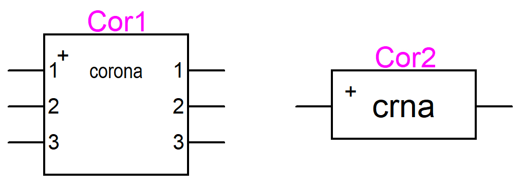
EMTP corona device symbols: the single-phase and three-phase nonlinear shunt-branch forms used to attach corona to a line section.
Figure 6 — Corona device symbols for single-phase and three-phase EMTP® implementation. The device is inserted as a nonlinear shunt branch associated with a line section — the single-phase form suits simplified single-conductor studies, the three-phase form is used where phase coupling and multiphase corona must be represented.

Section 10

Constant-parameter and frequency-dependent lines with corona

Corona can be combined with either line representation. A constant-parameter model uses parameters at one selected frequency and can be acceptable when a representative frequency suits the transient (a high frequency for fast fronts). A frequency-dependent model represents the variation of parameters with frequency and is generally more complete, because the frequency content of a surge changes as it propagates and higher-frequency components attenuate faster.

Once corona is active, it can dominate

When corona is included, the difference between constant-parameter and frequency-dependent lines can become less pronounced, because corona itself introduces strong nonlinear attenuation and front distortion — it can become one of the controlling effects. A frequency-dependent model remains more physically complete, but a frequency-dependent model without corona can still give an unrealistic waveform, because a major nonlinear damping mechanism is missing. Adding a more advanced linear line model does not remove the need for corona when the voltage exceeds inception. This is the key distinction across the series: in the simplified CIGRE backflashover calculation corona may be neglected with limited effect on the final rate (it barely changes the tail that drives leader progression), but in a detailed EMT surge-propagation study corona can be important because it changes the waveform that arrives at the insulation or substation.

Section 11

Field-test comparison: line model and corona

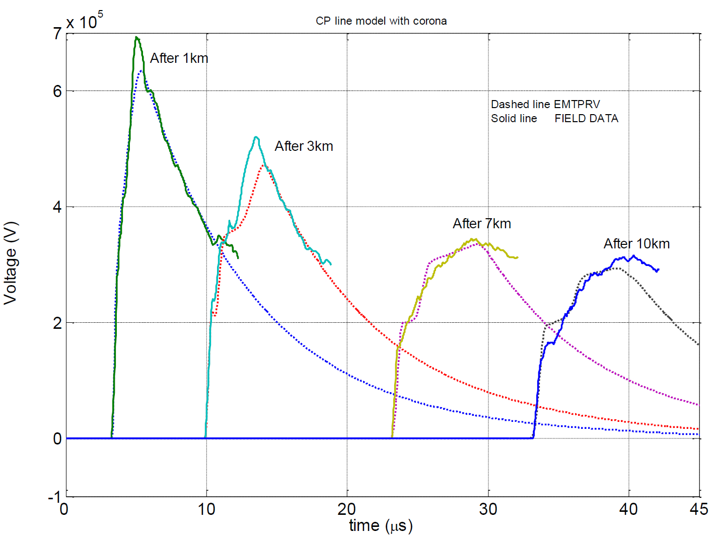
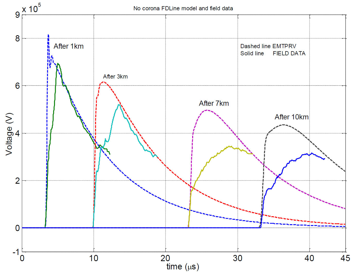
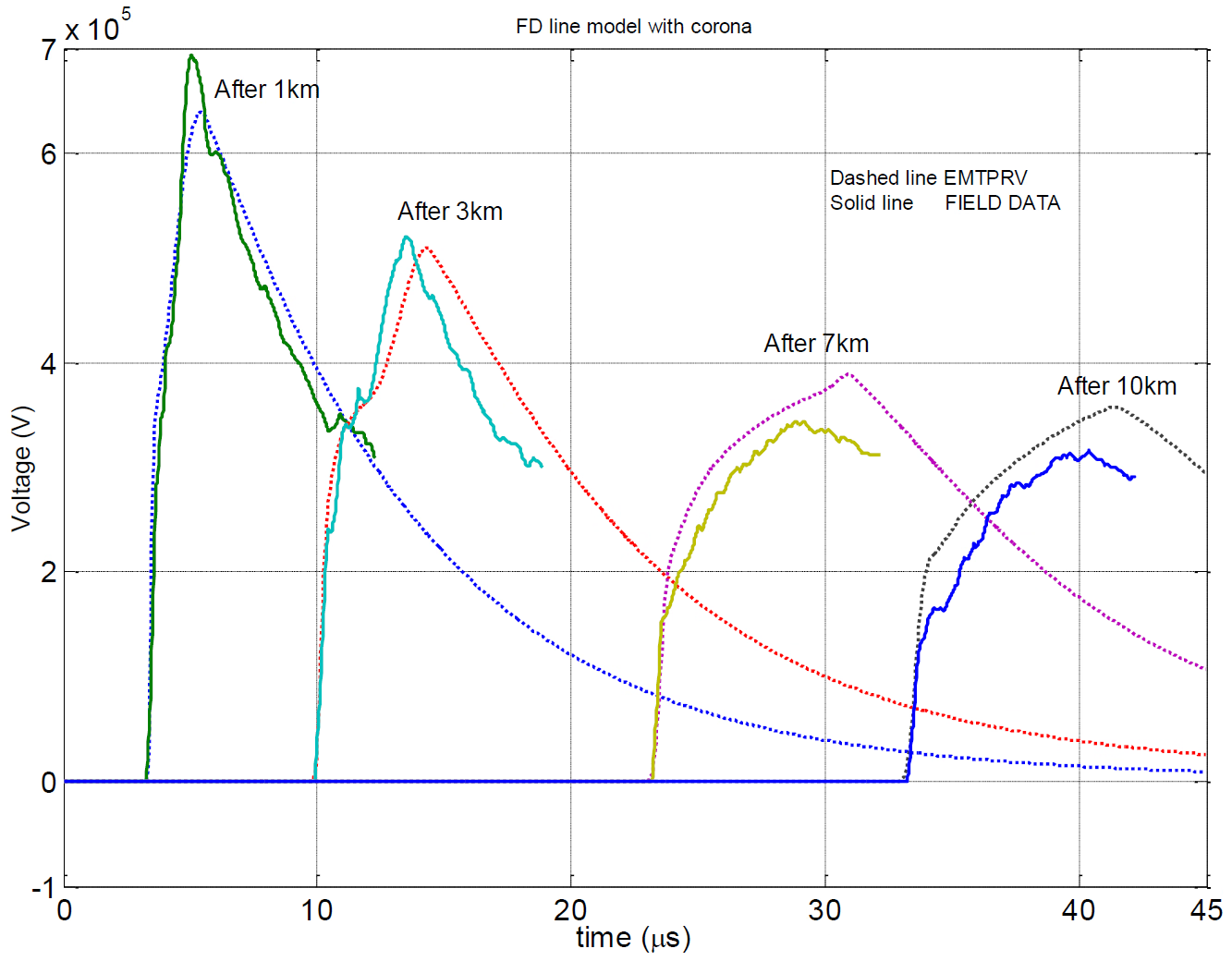
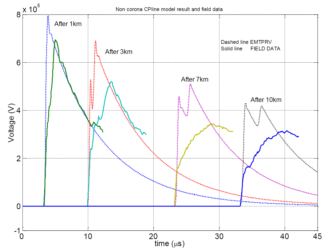
The four waveform comparisons below — from Gary’s field test, simulated with 100 kHz line data — isolate two modelling choices: the line-parameter representation (constant-parameter versus frequency-dependent) and the corona representation (absent versus the Suliciu model). Read the two effects from matched pairs: Figure 2 versus 3 (and 4 versus 5) isolates corona; Figure 2 versus 4 (and 3 versus 5) isolates frequency dependence. Note that corona also retards the front, not only lowers the peak.

Surge propagation: constant-parameter line at 100 kHz with no corona model; the simulated wave stays too steep and too high compared with the field measurement.
Figure 2 — Constant-parameter line, no corona. Propagation delay is broadly reproduced, but the wave stays too steep and too high versus the field data, increasingly so with distance.
Surge propagation: constant-parameter line at 100 kHz with the Suliciu corona model; the simulated wave is much closer to the field measurement, with reduced peak and steepness.
Figure 3 — Constant-parameter line with the Suliciu corona model. The peak is reduced, the front is less steep and the distortion grows with distance — much closer to the measured response.
Surge propagation: frequency-dependent line at 100 kHz with no corona model; better attenuation than the constant-parameter case but still over-steep and over-high.
Figure 4 — Frequency-dependent line, no corona. Attenuation and dispersion improve over the CP model, but the wave is still too steep and too high because the nonlinear effect is missing.
Surge propagation: frequency-dependent line at 100 kHz with the Suliciu corona model; the most physically complete match to the field measurement.
Figure 5 — Frequency-dependent line with the Suliciu corona model. Corona reduces the rate of rise and the peak while the FD line carries the distributed losses — the best agreement with this field test of the four cases shown.
What the comparison shows

A model without corona tends to overestimate the wave steepness and the peak voltage after propagation; adding corona brings both down and improves agreement with the measurement. Frequency dependence improves the linear propagation model, but it does not replace corona — once corona is active, the difference between the constant-parameter and frequency-dependent lines becomes less obvious. For real studies the lesson is direct: a more advanced line model is not a substitute for corona modelling if the conductor voltage exceeds inception. A single field test shows the best agreement here — it cannot by itself establish general completeness.

Section 12

When corona should be included

Consider corona when the conductor voltage may exceed inception and the resulting surge shape affects the engineering decision. Typical cases are lightning surge propagation, incoming surges at substations, switching overvoltages on long EHV lines, insulation-coordination studies near withstand limits, arrester energy and protective-level studies, high-overvoltage line energisation, and validation against field tests.

Corona is usually less important when the voltage stays below inception, when the study concerns low-frequency or temporary overvoltage behaviour, when the line section is too short for distortion to accumulate, or when a conservative no-corona estimate is intentionally used and clearly stated. Do not add corona automatically to every study — base the decision on voltage level, surge shape, line length, conductor geometry and objective.

Section 13

Corona and incoming-surge studies

One of the most important uses of corona modelling is the incoming surge to a substation. A lightning or switching surge may travel several kilometres before arriving, and corona reduces its steepness and peak along the way. This matters because substation insulation stress depends on the wave front and arrival time, not only the peak — steepness drives the volt–time flashover of gaps and insulators, the inter-turn stress in transformer windings, and arrester energy and timing. Neglecting corona usually makes the incoming surge more severe, so it is often a conservative simplification — but not unconditionally: it depends on the transient, geometry, weather, air density and corona model, and a changed front time can shift the surge relative to arrester operation or reflections. State the assumption when the result is near the withstand limit; where margins are tight, corona improves realism.

Section 14

Corona versus frequency-dependent line modelling

Corona and frequency dependence are different physical effects and should not be treated as alternatives. Frequency-dependent line modelling is a linear effect acting through the line’s series impedance — conductor skin effect, frequency-dependent earth return, modal propagation and distributed attenuation — and it is active at all voltage levels. Corona is a nonlinear shunt effect that becomes active only above the inception threshold. Both can reduce and distort a surge, but for different reasons, so a study may need both. The choice depends on whether accurate linear propagation, nonlinear corona behaviour, or both, control the result.

Section 15

Numerical behaviour and the data it needs

Corona is nonlinear and distributed, so the solver must reconcile the linear network and the nonlinear corona current at each time-step — computing the voltage, deciding whether corona is active, finding the corona charge and current, updating the equivalent injection and iterating to convergence. Expect a slower simulation, and choose the time-step and section length carefully. Very steep or discontinuous waves can cause numerical oscillation; if it appears, suspect an over-long section, an unsuitable time-step, poor corona parameters, an abrupt waveform discontinuity or insufficient numerical damping.

Data is the usual limitation

A corona model needs more than an ordinary line model: conductor radius, bundle and height data, phase spacing, ground resistivity, the capacitance matrix, the inception voltage or onset gradient, air-density and surface-irregularity factors, polarity, weather, the surge waveform, the section length and the corona-model parameters. A dynamic (Suliciu) model needs further parameters for the rate-dependent \(q\)–\(v\) behaviour — not found on a standard line schedule, and usually taken from experiment, literature, research data or calibration against field measurements. The model may be in the software while the data is the hard part.

Section 16

Checks and practical interpretation

Corona modelling should sharpen understanding, not create false precision: the result depends on assumptions about inception, weather, polarity, conductor condition and model parameters. Where the result is sensitive to those assumptions, say so — and consider showing both no-corona and with-corona cases. A no-corona model is often a useful conservative upper bound on propagated-surge steepness and peak, but not universally so — a changed front time can affect reflections, arrester operation and insulation-stress timing; a with-corona model gives a more realistic propagated waveform. Before relying on a corona model, confirm:

  • The expected conductor voltage exceeds corona inception.
  • The conductor radius and bundle data are correct, and the inception assumption suits weather, polarity and air density.
  • The line is subdivided with a section length suited to the surge rise time, and the capacitance matrix matches the section.
  • The time-step is small enough for the surge front and the corona dynamics.
  • The corona parameters rest on suitable data or documented assumptions.
  • The simulation stays numerically stable, with a physically reasonable reduction in steepness and peak.
  • The result is compared with field, laboratory or published data where possible.
  • The case is run with and without corona — the single most useful check of whether corona controls the result.

Section 17

Main takeaway

Main takeaway

Corona is a distributed, voltage-dependent nonlinear effect: above inception it raises the apparent capacitance, lowers velocity and surge impedance, and rounds and delays the front. The practical skill is knowing when it controls the result — lightning, incoming surges, long-line propagation, severe switching surges and field-test comparison — treating corona and a frequency-dependent line as complementary (a frequency-dependent model without corona can still overestimate steepness and peak), validating the Suliciu parameters, and stating whether corona is included with its inception assumptions, segmentation and the result’s sensitivity to them.

References

References

The standards, technical brochures, key papers and reference works behind this page.

  1. J. A. Martinez-Velasco, Ed., Power System Transients: Parameter Determination. Boca Raton, FL, USA: CRC Press, 2010.
  2. A. R. Hileman, Insulation Coordination for Power Systems. New York, NY, USA: Marcel Dekker, 1999.
  3. F. W. Peek, Dielectric Phenomena in High Voltage Engineering, 3rd ed. New York, NY, USA: McGraw-Hill, 1929.
  4. CIGRE Working Group 33.07, Guidelines for the Evaluation of the Dielectric Strength of External Insulation, Technical Brochure 72. Paris, France: CIGRE, 1992.
  5. IEEE Std 1243-1997, IEEE Guide for Improving the Lightning Performance of Transmission Lines. New York, NY, USA: IEEE, 1997.
  6. CIGRE Working Group C4.23, Procedures for Estimating the Lightning Performance of Transmission Lines – New Aspects, Technical Brochure 839. Paris, France: CIGRE, 2021.
  7. EMTP® software documentation and built-in Help.

Sixteen-Part Technical Series

EMTP® Line, Cable & Lightning Modelling

A sixteen-part guide spanning line and cable modelling, overhead-line physics, lightning, and the dielectric strength of external insulation.

Part 7 Reading now

Corona Effect in EMTP® Overhead Lines

How corona attenuates and distorts travelling surges, and the q–v and distributed nonlinear models.

Series progress 7 of 16