Lightning Grounding · CDEGS HIFREQ

Frequency-Dependent Soil and Tower-Footing Electrode Modelling in HIFREQ

High-frequency grounding studies need a different view of soil and earthing electrodes from power-frequency earthing. At 50/60 Hz an electrode is often a single low-frequency resistance — adequate for earth-potential-rise, touch and step studies, but not for lightning. A lightning current is broadband: in the first microseconds the electrode is not equipotential, current propagates along buried conductors, soil capacitance matters, and soil resistivity and permittivity change with frequency. This guide covers how to represent that behaviour — impulse impedance, frequency-dependent soil and the CDEGS HIFREQ options — and when simplified formulas are enough versus a full physical model.

Reading time ≈ 28 min · HIFREQ grounding guide

Lightning and fast-front grounding studies ask a different question from conventional power-frequency earthing. A power-frequency earth assessment — earth potential rise, touch and step voltage — can often use a single low-frequency resistance. A lightning study cannot: the current is broadband, and during its first microseconds the tower footing or earth electrode behaves as a high-frequency distributed system, not a single equipotential object. Current propagates along the buried conductors, voltage drops occur along the electrode, soil capacitance becomes relevant, and the soil’s own resistivity and permittivity change with frequency. So whenever lightning performance, backflashover, transferred voltage or transient grounding impedance is being assessed, the electrode and soil should be treated at high frequency.

In CDEGS this is normally done with the HIFREQ module, which represents the earthing system, buried conductors, soil layers and nearby metallic systems with their real geometry — important because the simplified equations are valid only for idealised electrodes (a single counterpoise, a rod, a four-leg star) in uniform soil. The practical principle: use simplified formulas for first estimates, screening and understanding; use HIFREQ (or an equivalent electromagnetic model) for detailed studies, non-standard geometry, multilayer soil, nearby metalwork, transferred voltage and safety-critical conclusions. This page is part of the APS lightning and grounding series alongside the impulse resistance of ground electrodes, tower modelling for lightning and CIGRE backflashover notes.

Abbreviations used on this page

HIFREQCDEGS high-frequency electromagnetic module

CDEGSSES grounding / electromagnetic software suite

\(R_{LF}\)Low-frequency footing resistance

\(Z_P\)Impulse impedance

ICImpulse coefficient, \(Z_P/R_{LF}\)

\(l_{EF}\)Effective length of the counterpoise / electrode

\(\rho(f),\ \varepsilon_r(f)\)Frequency-dependent resistivity / relative permittivity

\(\rho_0\)Low-frequency (100 Hz reference) resistivity

GPRGrounding potential rise

\(E_0\)Critical soil-ionisation electric field, kV/m (soil breakdown in the ground — not the air-gap leader-inception gradient used on other pages)

SESSafe Engineering Services — CDEGS developer

TBCIGRE Technical Brochure (e.g. TB 839)

Key idea

At lightning frequencies an earth electrode is a distributed, lossy system, not a single resistance — describe it by its impulse impedance \(Z_P=V_P/I_P\) (peak electrode voltage over peak injected current). And \(Z_P\) is not always larger than the low-frequency resistance.
Soil is frequency-dependent: \(\rho\) falls and \(\varepsilon_r\) changes with frequency (Alipio–Visacro), so a constant low-frequency soil model can overestimate the transient GPR — strongest in high-resistivity soil and for fast fronts.
For screening use impulse impedance, the impulse coefficient and effective counterpoise length; for complex geometry, multilayer soil or safety-critical work, model the electrode physically in HIFREQ with frequency-dependent soil.
Do not add soil ionisation as a default favourable correction — its time lag can make it non-conservative for backflashover. Treat it only as a validated sensitivity case.

Key terms used on this page

01Impulse impedance, \(Z_P\)

Peak electrode voltage divided by peak injected current, \(Z_P=V_P/I_P\); the lightning-frequency equivalent of footing resistance.

02Impulse coefficient, IC

\(IC=Z_P/R_{LF}\); below 1 when the impulse impedance is lower than the low-frequency resistance.

03Effective length, \(l_{EF}\)

The electrode length beyond which extra conductor does little to reduce the peak voltage under a lightning impulse.

04Frequency-dependent soil

Soil whose resistivity and permittivity vary with frequency over the lightning band, rather than being constant.

05Alipio–Visacro model

Measured empirical (and causal) relations giving \(\rho(f)\) and \(\varepsilon_r(f)\) from the low-frequency resistivity.

06Causal soil model

A semi-theoretical Alipio–Visacro form linking conductivity and permittivity consistently, with mean/conservative levels.

07Soil ionisation

Local soil breakdown at high field that enlarges the effective electrode and lowers apparent resistance — a nonlinear, time-dependent effect.

08Transient grounding impedance

The electrode’s voltage-to-current behaviour under a fast-front current, frequency- and time-dependent.

09Grounding potential rise (GPR)

The voltage of the earthing system relative to remote earth during current injection.

10Counterpoise

A buried horizontal earth conductor (often in arms from the tower) used to lower footing impedance.

11Low-frequency resistance, \(R_{LF}\)

The electrode’s dissipation resistance when it is essentially equipotential — the conventional measured footing resistance.

12CDEGS HIFREQ

The SES electromagnetic module that solves buried-conductor and soil-layer geometry over frequency.

Section 1

Why high-frequency footing behaviour matters

The voltage differences that develop along an electrode and between the electrode and remote earth are what stress the insulation in a backflashover or transferred-voltage event. At power frequency the whole electrode is essentially at one potential, so a single resistance describes it. Under a lightning current the picture changes within the first microseconds: the surge enters at one point, travels along the buried conductors, and leaks continuously into the soil. The far end of a long counterpoise may add little, because the surge is largely attenuated before it gets there. The electrode therefore has a frequency- and time-dependent response, and a single low-frequency resistance does not capture it.

Section 2

Why low-frequency footing resistance is not enough

The low-frequency footing resistance \(R_{LF}\) describes the electrode when it can be assumed almost equipotential — true at low frequency because the inductive and capacitive effects of the buried conductors are small compared with the dissipation resistance into soil. At lightning frequencies the electrode behaves more like a lossy transmission line: a current impulse entering one end travels along the conductor and leaks into the soil as it propagates. The response is better described by the impulse impedance:

\[ Z_P=\frac{V_P}{I_P} \]

\(Z_P\): impulse impedance
\(V_P\): peak voltage rise of the electrode
\(I_P\): peak injected current

\(V_P\) and \(I_P\) are peak values that need not occur at the same instant; the impulse impedance is conventionally the ratio of their peaks. Crucially, \(Z_P\) is not always larger than \(R_{LF}\). For a short electrode in low-resistivity soil, inductive behaviour can make \(Z_P\ge R_{LF}\); but in high-resistivity soil the frequency dependence of the soil (resistivity falling with frequency) reduces the GPR, so \(Z_P\) can fall below \(R_{LF}\) — the effect being stronger for subsequent strokes. The old rule that lightning impulse impedance is always higher than the measured footing resistance is therefore not generally correct.

Section 3

Soil as a frequency-dependent medium

In high-frequency studies, soil is a dispersive material — its resistivity \(\rho(f)\) and relative permittivity \(\varepsilon_r(f)\) both vary over the frequency range of lightning currents. The field measurements of Visacro and Alipio showed that, in general, resistivity decreases as frequency rises while permittivity also changes with frequency. This affects the calculated grounding potential rise and transient impedance: a constant-parameter soil model (using the low-frequency \(\rho_0\) across the whole spectrum) tends to overestimate the voltage rise compared with a frequency-dependent model, most noticeably in high-resistivity soils and for fast-front currents. At power frequency the two models coincide, so the divergence is specifically a fast-front phenomenon.

Frequency-dependent soil is therefore recommended for lightning-current injection into footings, transient grounding impedance, backflashover, GPR during fast-front events, transferred voltage, substation or tower earthing response at high frequency, and comparison with measured impulse response.

Section 4

The Alipio–Visacro empirical soil model

The Alipio–Visacro empirical model gives simple, practical equations for frequency-dependent resistivity and permittivity from the resistivity at 100 Hz (the physically consistent causal form follows in the next section). The mean-tendency resistivity expression, normalised so that \(\rho(100\,\text{Hz})=\rho_0\), is:

\[ \rho(f)=\frac{\rho_0}{1+\left(1.2\times10^{-6}\,\rho_0^{0.73}\right)\left(f^{0.65}-100^{0.65}\right)} \]

\(\rho(f)\): soil resistivity at frequency \(f\), \(\Omega\cdot\text{m}\)
\(\rho_0\): soil resistivity at 100 Hz, \(\Omega\cdot\text{m}\)
\(f\): frequency, Hz

The frequency dependence acts on \(f^{0.65}\) with the 100 Hz value subtracted, so the expression is normalised to 100 Hz: at \(f=100\) the bracket is zero and \(\rho=\rho_0\); as \(f\) rises the denominator grows and the resistivity falls. Different references and software help files may present this 100 Hz normalisation in slightly different notations — the essential requirement is that the expression returns \(\rho(100\,\text{Hz})=\rho_0\). The form above is written so that the 100 Hz reference is explicit; confirm the exact notation against your CDEGS help file or source before quoting coefficients.

The companion relative-permittivity expression is:

\[ \varepsilon_r(f)=7.6\times10^{3}\,f^{-0.4}+1.3 \qquad\qquad \mu_r=1 \]

\(\varepsilon_r(f)\): relative permittivity at frequency \(f\)
\(f\): frequency, Hz
\(\mu_r\): relative permeability (kept at unity)

This is a mean-tendency fit; it is meaningful in the higher-frequency range. At power frequency it predicts a very large \(\varepsilon_r\), but the displacement-current contribution there is negligible, so it does not matter. Keeping \(\mu_r=1\) treats soil as electrically dispersive but not magnetic — appropriate unless a ferromagnetic material is being modelled. The model changes the electrical properties of each layer with frequency; it does not change the soil layering or thicknesses.

Section 5

The Alipio–Visacro causal model

The simple empirical equations were intentionally fitted conservatively, so strict causality between resistivity and permittivity is not fully preserved. A later, semi-theoretical causal Alipio–Visacro model links the frequency variation of conductivity and permittivity in a physically consistent (Kramers–Kronig) way, and is usually written in terms of conductivity:

\[ \sigma(f)=\sigma_0+\sigma_0\,h(\sigma_0)\left(\frac{f}{1\,\text{MHz}}\right)^{\xi},\qquad \sigma=\frac{1}{\rho} \]

\(f\): frequency, Hz (used consistently with the \(f/1\,\text{MHz}\) normalisation)
\(\sigma(f)\): soil conductivity at frequency \(f\)
\(\sigma_0\): DC / low-frequency conductivity
\(h(\sigma_0)\): soil-dependent coefficient
\(\xi\): exponent (normalised at 1 MHz)

Because \(\sigma=1/\rho\), conductivity rising with frequency means resistivity falling with frequency. The model is based on measurements over roughly 100 Hz to a few MHz and offers mean, relatively conservative and conservative parameter sets — useful because real soil is never perfectly uniform.

What “conservative” means here

Frequency-dependent soil usually reduces the calculated transient grounding voltage versus constant soil. A “conservative” frequency-dependent model is therefore one that avoids exaggerating that reduction — it does not mean a higher soil resistance in the power-frequency sense. For routine work the automatic CIGRE–Visacro option is practical; for a specific causal model, the User-Defined option (Section 6) lets you enter calculated parameters at selected frequencies.

Section 6

Frequency-dependent soil in CDEGS HIFREQ: two options

HIFREQ offers two ways to represent frequency-dependent soil — the automatic CIGRE–Visacro et al. method and a User-Defined table. In both, the soil geometry and layer thicknesses stay part of the model; what changes with frequency is the electrical property of each layer.

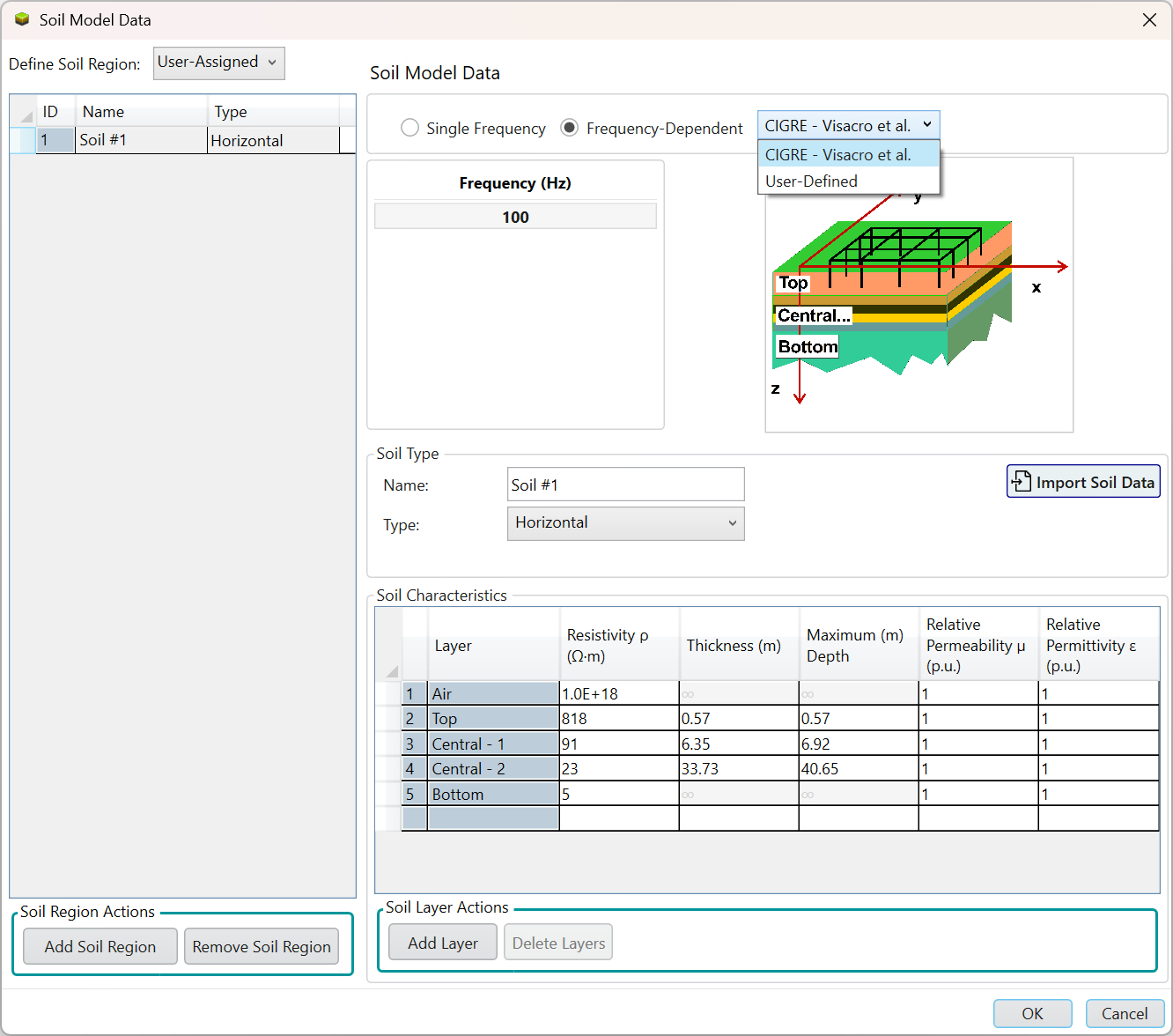
CDEGS HIFREQ Soil Model Data dialog with the Frequency-Dependent option set to the CIGRE-Visacro et al. method, and a horizontal multilayer soil table (Air, Top, Central-1, Central-2, Bottom) listing resistivity, thickness, permeability and permittivity per layer. — **Figure 1 —** The CDEGS HIFREQ *Soil Model Data* dialog. **Frequency-Dependent** soil is selected with the **CIGRE–Visacro et al.** method; each layer’s entered resistivity is taken as that layer’s low-frequency reference, and HIFREQ computes \(\rho(f)\) and \(\varepsilon_r(f)\) for every layer at each calculation frequency. The layering and thicknesses do not change with frequency — only the electrical properties. (The layer values shown are from one example soil model and are illustrative only.)

With the CIGRE–Visacro option the engineer enters the usual layered soil model, and the program takes each layer’s entered resistivity as the low-frequency reference (the Alipio–Visacro relations are normalised to 100 Hz); for each HIFREQ calculation frequency it computes that layer’s \(\rho(f)\) and \(\varepsilon_r(f)\). It suits the common case where a conventional low-frequency soil model is available but measured frequency-dependent data are not. With the User-Defined option the engineer enters soil properties at selected frequencies (for example 100 Hz, 1 kHz, 10 kHz, 100 kHz, 1 MHz) and the software interpolates between them; outside the entered range it extrapolates per its documented rule (confirm the exact behaviour for your installed version). It suits measured data, project-specific or client-specified tables, or a manually implemented causal model. State the frequency range the HIFREQ study needs — set by the chosen lightning-current waveform — and make sure the User-Defined table covers it, so the result does not rely heavily on extrapolation beyond the entered frequencies.

Which to use

Use CIGRE–Visacro when a recognised automatic method is needed and only the low-frequency (100 Hz) soil model is available. Use User-Defined when reliable measured or calculated frequency-dependent parameters exist or a specific model must be implemented — but not with arbitrary values, since a more detailed-looking table built on unreliable data is less, not more, defensible.

Section 7

The earth electrode as a distributed system

A buried counterpoise or footing electrode is a distributed circuit: along the conductor there is series resistance and inductance; from the conductor into the soil there is dissipation resistance and capacitance. So the electrode response is frequency-dependent even if the soil is assumed constant. Put simply: even with constant soil properties, a long buried electrode is not equipotential during a lightning impulse. At low frequency the inductance and capacitance are not dominant and the electrode behaves mainly as a resistance. At high frequency the conductor is no longer equipotential: the current wave travels along the electrode, loses energy into the soil and produces voltage differences along the conductor, so the electrode can appear capacitive over one band and inductive over another. The lightning current peak may occur before the electrode has reached its low-frequency behaviour — which is exactly why a single \(R_{LF}\) is not enough, and why, where the result matters, the electrode should be represented physically in HIFREQ with its real conductor lengths, burial depths, interconnections, soil layers and nearby metalwork.

Section 8

Simplified lightning-performance: impulse impedance

For transmission-line lightning-performance studies, CIGRE TB 839 notes that a simplified representation based on the first-stroke impulse impedance \(Z_P\) is accurate enough for many practical cases — useful because modelling every footing physically is heavy for long outage-rate studies. For a four-leg counterpoise, a first estimate of \(Z_P\) is:

\[ Z_P = 0.16\,\rho_0\,l^{-0.687} \quad (100\le\rho_0\le 600\ \Omega\cdot\text{m}) \] \[ Z_P = 0.4\,\rho_0^{0.89}\,l^{-0.75} \quad (600\le\rho_0\le 4000\ \Omega\cdot\text{m}) \]

\(Z_P\): impulse impedance, \(\Omega\)
\(\rho_0\): low-frequency soil resistivity, \(\Omega\cdot\text{m}\)
\(l\): average length of each counterpoise arm (per arm), m — not the total installed conductor length of all arms

These engineering expressions (Visacro / Silveira) apply to the first-return-stroke waveshape and to arm lengths \(l\) within the effective length; do not extrapolate beyond the stated resistivity ranges. They are arrangement-specific — they should not be applied directly to rods, meshes, irregular tower footings, multilayer soil or nearby buried metallic systems without validation. For other counterpoise arrangements a correction factor can be used for screening, but it is approximate — burial depth, interconnection and geometry strongly influence the response, so they are not a substitute for HIFREQ when the geometry is non-standard or the result is sensitive.

Section 9

The impulse coefficient method

When the low-frequency footing resistance is known, the impulse impedance can be estimated through the impulse coefficient:

\[ IC=\frac{Z_P}{R_{LF}} \qquad IC \approx 0.89-5\times10^{-5}\,\rho_0 \qquad Z_P=IC\times R_{LF} \]

\(IC\): impulse coefficient
\(Z_P\): impulse impedance, \(\Omega\)
\(R_{LF}\): low-frequency resistance of the electrode, \(\Omega\)
\(\rho_0\): low-frequency soil resistivity, \(\Omega\cdot\text{m}\)

The closed-form estimate applies to electrodes shorter than the effective length. For such electrodes the impulse impedance is below the low-frequency resistance, so \(IC<1\), and it falls further as resistivity rises (a stronger frequency-dependent-soil reduction in more resistive ground) — consistent with the \(Z_P<R_{LF}\) behaviour noted in Section 2. (Confirm the exact intercept and slope against your CIGRE TB 839 / Visacro source, and use \(IC=Z_P/R_{LF}\) directly with the Section 8 \(Z_P\) where the closed form does not apply.) The method is useful when \(R_{LF}\) is measured or calculated and the electrode is not longer than its effective length, and it avoids electrode formulas that may not match the real arrangement.

Section 10

Effective length of counterpoise electrodes

For lightning currents, lengthening a counterpoise does not keep reducing the peak tower voltage: beyond a limiting effective length \(l_{EF}\) the extra conductor contributes little, because the surge has already attenuated before reaching it. First estimates are:

\[ l_{EF}=17+0.042\,\rho_0-2\times10^{-6}\,\rho_0^{2} \quad\text{(first strokes)} \] \[ l_{EF}=9+0.021\,\rho_0-1\times10^{-6}\,\rho_0^{2} \quad\text{(subsequent strokes)} \]

\(l_{EF}\): effective length of the counterpoise / electrode, m
\(\rho_0\): low-frequency soil resistivity, \(\Omega\cdot\text{m}\)

The effective length is shorter for subsequent strokes because their shorter front time (~0.5–0.7 µs versus ~3.8 µs for the first stroke) means higher-frequency content, which attenuates faster along the buried conductor. Practically: for low-frequency resistance a longer electrode keeps helping, but for lightning impulse response, length beyond \(l_{EF}\) gives little improvement — important for economical footing design, since a very long counterpoise may cut the measured \(R_{LF}\) without improving lightning performance.

Section 11

When simplified methods are acceptable

Simplified \(Z_P\), impulse-coefficient and effective-length methods are acceptable for early design screening, comparing footing options, judging whether a measured footing resistance is likely adequate, transmission-line outage-rate calculations where many towers must be represented, and explaining the difference between \(R_{LF}\), \(Z_P\) and effective length.

When they are not sufficient

They are not enough when the electrode geometry is complex, the soil is strongly multilayered or laterally variable, nearby metallic systems affect the result, transferred voltage is assessed, a substation earthing grid is involved, footing conductors have unusual geometry, or the result feeds detailed design or safety-critical conclusions. For those cases, model the electrode physically in CDEGS HIFREQ.

Section 12

Soil ionisation: what it means

Soil ionisation occurs when the field around an electrode is high enough to break the soil down locally: conducting channels form in the soil voids, effectively enlarging the electrode radius and surface area and reducing the apparent resistance. Older lightning-performance methods often included it because it appears to reduce footing resistance during high-current injection — the higher the injected current, the more conductive the nearby soil and the lower the footing resistance (the existing APS note on the impulse resistance of ground electrodes develops the hemispherical \(R_i=R_0\sqrt{I_g/I}\) treatment). The effect is physically real, but its simplified representation is problematic.

Simplified ionisation models usually assume the resistance reduction follows the injected current directly. Measurements and detailed studies, however, show that ionisation and de-ionisation take time: the maximum ionised region and minimum resistance may occur after the lightning-current peak, not at it. That timing is critical for backflashover, where the maximum insulator voltage is associated with the peak or steep front of the current.

Section 13

Why soil ionisation should not be included by default

For routine transmission-line lightning-performance studies, soil ionisation should not normally be included by default in simplified calculations. First, simplified models apply a quasi-static \(R(I)\) curve without the ionisation/de-ionisation time lag, so they can reduce the footing resistance too early — lowering the resistive voltage at the instant of peak current and so under-predicting peak tower voltage and backflashover risk. That is not conservative, and it matters most on fast-front first strokes. Second, ionisation is strongest for small, concentrated electrodes with high current density; many footings have a larger effective perimeter (counterpoise or foundation systems) where the field may not be high enough over a wide region at the time of peak voltage. Third, high-resistivity soils usually need longer or larger electrodes, which reduce current density and limit ionisation; low-resistivity soils may ionise more easily but their base lightning performance is often already acceptable. Fourth, frequency-dependent soil and impulse impedance already capture much of the real high-frequency response, so adding simplified ionisation on top can double-count favourable effects.

Recommended approach

Use frequency-dependent soil and impulse impedance for simplified lightning-performance calculations, and do not include soil ionisation by default. Note that frequency-dependent soil (a linear, dispersion effect) and ionisation (a nonlinear, current-amplitude effect) are different physics — one is not a substitute for the other. Consider ionisation only as a sensitivity case, or when a validated time-dependent nonlinear model and site-specific data are available; do not use simplified ionisation as the main basis for peak insulator voltage or backflashover assessment.

Section 14

If soil ionisation must be considered

If a project specifically requires ionisation to be investigated, it should not be applied blindly using \(R_{LF}\). A better simplified approach starts from the impulse impedance \(Z_P\): if a legacy ionisation formula is used, replacing \(R_{LF}\) with \(Z_P\) is more consistent with lightning-frequency behaviour. The critical field \(E_0\) should be chosen carefully — it is commonly taken as about 300–400 kV/m for design (IEEE/CIGRE), but reported values span roughly 300 kV/m to over 1000 kV/m and are soil-dependent, so \(E_0\) is best treated as an uncertain sensitivity parameter (with local measurement where the result is important) rather than a fixed constant. Even then, present the result as a sensitivity case, not the main design case, unless the model represents time-dependent ionisation and is validated.

Suggested report statement

“Soil ionisation was not included in the base case because simplified ionisation models can overestimate the favourable reduction in electrode impedance at the time of peak lightning current. The base model used frequency-dependent soil and an impulse-electrode response. Soil ionisation, if considered, is treated only as a sensitivity case unless supported by a validated time-dependent model or site-specific measurements.”

Section 15

How frequency-dependent soil affects the results

With frequency-dependent soil the grounding response can differ significantly from a constant-soil result. The common effects are a lower high-frequency soil resistivity, a different capacitive behaviour through \(\varepsilon_r(f)\), a lower transient grounding impedance in many high-resistivity soils, a lower calculated GPR for fast-front injection, a different current distribution along counterpoise electrodes, and a different footing impulse response.

Compare both models

This does not mean frequency-dependent soil always gives a “safer” result — it gives a more realistic representation over the lightning band, provided the base soil model is correct. For important studies, run both constant and frequency-dependent soil and see whether the frequency-dependent model is controlling the result.

Section 16

Practical HIFREQ modelling guidance

Where the result is important, represent the footing or earthing electrode physically in HIFREQ rather than as a single resistance. Include the conductor geometry, counterpoise length and orientation, burial depth and radius, interconnections and tower-footing connections, soil layering, frequency-dependent soil properties, nearby buried metallic systems where relevant, and the frequency range required to represent the lightning-current front or injected waveform (set by the lightning & switching current waveform chosen for the study). Confirm:

The electrode is modelled with its real geometry, not only an equivalent resistance, wherever the result matters.
Frequency-dependent soil is used for lightning, fast-front, impulse-impedance, transferred-voltage and high-frequency GPR studies.
CIGRE–Visacro soil is used when only a low-frequency soil interpretation is available; User-Defined when reliable measured or calculated frequency-dependent values exist.
Arrangement-specific hand formulas are not used as a substitute for HIFREQ where geometry, soil layering or nearby metalwork differ from the simplified assumptions.
Simplified impulse-impedance / impulse-coefficient / effective-length methods are used only where their assumptions hold; final modelling uses HIFREQ with the actual geometry and soil.
Soil ionisation is excluded from the base case and, if used at all, is a clearly labelled, validated sensitivity case.

Section 17

Main takeaway

For lightning and HIFREQ studies, a tower-footing electrode should not be represented only by its low-frequency resistance. The electrode has a frequency- and time-dependent response because the buried conductor behaves as a distributed lossy system and because soil resistivity and permittivity vary with frequency.

Engineering conclusion

For simplified transmission-line lightning-performance work, the first-stroke impulse impedance \(Z_P\), the impulse coefficient \(IC\) and the effective length \(l_{EF}\) are practical tools for screening and outage-rate studies — but not substitutes for detailed HIFREQ modelling of complex electrodes and multilayer soil. For accurate results use CDEGS HIFREQ (or an equivalent electromagnetic model) with physical electrode geometry and frequency-dependent soil; do not include simplified soil ionisation in the base case unless a validated time-dependent model is available. The modern practical approach is to model frequency-dependent soil and impulse-electrode behaviour correctly, and to treat soil ionisation only as a justified sensitivity case rather than a default favourable correction.

References

The standards, technical brochures, key papers and reference works behind this page.

CIGRE Working Group C4.33, Impact of Soil-Parameter Frequency Dependence on the Response of Grounding Electrodes and on the Lightning Performance of Electrical Systems, Technical Brochure 781. Paris, France: CIGRE, 2019.
S. Visacro and R. Alipio, “Frequency dependence of soil parameters: Experimental results, predicting formula and influence on the lightning response of grounding electrodes,” IEEE Transactions on Power Delivery, vol. 27, no. 2, pp. 927–935, Apr. 2012.
R. Alipio and S. Visacro, “Frequency dependence of soil parameters: Effect on the lightning response of grounding electrodes,” IEEE Transactions on Electromagnetic Compatibility, vol. 55, no. 1, pp. 132–139, Feb. 2013.
R. Alipio and S. Visacro, “Modeling the frequency dependence of electrical parameters of soil,” IEEE Transactions on Electromagnetic Compatibility, vol. 56, no. 5, pp. 1163–1171, Oct. 2014.
CIGRE Working Group C4.23, Procedures for Estimating the Lightning Performance of Transmission Lines – New Aspects, Technical Brochure 839. Paris, France: CIGRE, 2021.
J. A. Martinez-Velasco, Ed., Power System Transients: Parameter Determination. Boca Raton, FL, USA: CRC Press, 2010.
CDEGS Software Package (Current Distribution, Electromagnetic Fields, Grounding and Soil Structure Analysis), Safe Engineering Services Ltd., Canada.

Part 11 Reading now

Frequency-Dependent Soil & Tower-Footing in HIFREQ

Impulse impedance, the Alipio–Visacro soil model and effective counterpoise length in CDEGS HIFREQ.

Series progress 11 of 16

Part 12

Impulse Resistance of Ground Electrodes

How footing resistance changes under lightning current — soil ionisation and the impulse-resistance model.