EMTP® Line & Cable Modelling

Modelling of Cables and Overhead Lines in EMTP®

A transmission line or cable is not a single series impedance — it is a distributed electromagnetic system whose resistance, inductance, conductance and capacitance change with frequency, geometry, earth return and bonding. This guide explains the five EMTP® line/cable models — CP, FD, Wideband, Exact-PI and Nominal-PI — how each one solves the line equations, what it assumes, and how to enter the conductor geometry, soil and material data that drive the result.

Reading time ≈ 30 min · EMTP® modelling guide

In an electromagnetic transient (EMT) study, the overhead line or cable is often the component that decides the answer. It sets the surge impedance that shapes a travelling wave, the resonance that amplifies a switching or harmonic event, the attenuation that damps it, and the delay that governs reflections. Because its parameters are distributed along the route and frequency dependent, the same physical line can require very different mathematical models depending on what is being studied.

EMTP® provides a single Line/Cable Data device that calculates the per-unit-length parameters from conductor geometry and material properties, and then builds one of five models from them: the Constant Parameter (CP), Frequency Dependent (FD), Wideband (WB), Exact-PI and Nominal-PI models. This guide explains what each model represents, the assumptions behind it, when it is the right choice, and how the underlying conductor, soil and material data are entered so that the computed model is physically meaningful.

Abbreviations used on this page

EMTP®Electromagnetic Transients Program

EMTElectromagnetic transient

OHLOverhead line

CPConstant Parameter model

FDFrequency Dependent modelnot frequency-domain

WBWideband model

PIEquivalent circuit — one series branch, two shunt branches

p.u.l.Per-unit-length

SC cableSingle-core cable

PT cablePipe-type cable

HVDCHigh-voltage direct current

GISGas-insulated switchgear

FDCMFrequency Dependent Cable Model correction

Key idea

A line or cable is a distributed, frequency-dependent system; the model must match the transient and frequency range being studied.
CP and FD solve in the modal domain (real transformation matrix); WB solves in the phase domain with full frequency dependence.
WB is the most accurate time-domain model and the default for cables, HVDC, mixed and unbalanced systems; Exact-PI is a frequency-domain reference; Nominal-PI is a simple steady-state equivalent.
The model is only as good as the input data — geometry, sheaths, semiconducting layers, soil and bonding all change the result.

Key terms used on this page

01Per-unit-length (p.u.l.)

Series impedance \(Z'\) and shunt admittance \(Y'\) defined per metre of line, as matrices for a multi-conductor system.

02Characteristic impedance, \(Z_c\)

The impedance relating the voltage and current of a travelling wave; \(Z_c=\sqrt{Z'/Y'}\).

03Propagation constant, \(\Gamma\)

Carries the attenuation and phase shift of a wave along the line; \(\Gamma=\sqrt{Z'Y'}\).

04Modal domain

A decoupled representation in which each propagation mode is solved separately, using a transformation matrix.

05Phase domain

The coupled conductor representation solved directly, retaining all inter-conductor coupling (used by WB).

06Transformation matrix, \(T_i\)

Also called the Q matrix; converts phase quantities to modal quantities. Generally complex; CP/FD need a real approximation.

07Vector fitting

A rational-function fitting technique used by WB to build a time-domain model of \(Y_c\) and the propagation function \(H\).

08Passivity

A fitted model is passive if it cannot generate energy; a non-passive WB fit can cause numerical instability.

09Loss factor, \(\tan\delta\)

Dielectric loss of the insulation; the ratio of the imaginary to the real part of the complex permittivity.

10Cross-bonding

Transposing cable sheaths between minor sections so the induced sheath voltages tend to cancel over a major section.

11Skin & proximity effect

Frequency-dependent crowding of current within a conductor (skin) and due to nearby conductors (proximity).

12DC correction

A WB option that improves accuracy near DC without making the whole fitting band excessively stiff — important for HVDC.

Section 1

Why the choice of model matters

Different transient studies demand different levels of detail. A short lightning surge contains very-high-frequency content: skin effect alters the current distribution within a conductor, proximity effect alters it between nearby conductors, the earth-return path changes with frequency, dielectric losses become relevant, and sheaths, screens, armour, pipes and bonding all influence the result. A load-flow or fundamental-frequency study needs none of this — a simple PI model is enough.

The modelling method should therefore be chosen against the type of study and the frequency range; the required accuracy and the line or cable length; whether the system is balanced or unbalanced; whether it is an overhead line, underground cable, submarine cable, pipe-type cable or a combined system; whether the result is sensitive to propagation delay; whether high-frequency earth return must be represented; whether sheath, screen, armour or pipe currents matter; and whether near-DC accuracy is required, as in HVDC studies.

Overhead lines versus cables

Overhead lines are bare conductors in air; their behaviour is governed by conductor height, phase spacing, shield-wire position, bundling, tower geometry, the earth-return path, transposition and ground resistivity. Because the insulation is air, the shunt capacitance is comparatively low, but lines can be very long, so wave propagation, reflections and travelling-wave behaviour dominate.

Cables are geometrically more complex — a single-core cable may carry a core, conductor screen, insulation, insulation screen, metallic sheath, armour and an outer serving, all within soil, duct, tunnel or water. Cable results are sensitive to insulation permittivity and loss factor, sheath bonding and cross-bonding, proximity and skin effect, earth return, multilayer soil, semiconducting layers and — for HVDC — near-DC accuracy. Because cables have much higher capacitance than lines, cable energisation, resonance, sheath voltages and HVDC transients all demand careful modelling. For the cable-specific workflow — Cable Constants conversion, sheath and screen treatment, bonding and cross-bonding, armour and validation — see EMTP Modelling of Insulated Power Cables.

Section 2

The distributed-parameter line equations

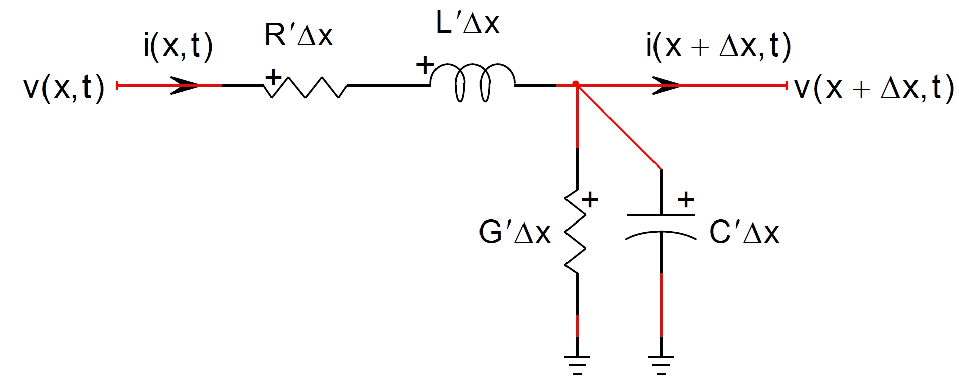
Every EMTP® line/cable model is built from the same physics. Consider a short element of a single conductor of length \(\Delta x\). Its equivalent circuit contains a series resistance and inductance and a shunt conductance and capacitance, each per unit length.

Lumped-element equivalent circuit of a transmission-line section of length delta-x, with series R'-delta-x and L'-delta-x and shunt G'-delta-x and C'-delta-x between v(x,t) and v(x+delta-x,t). — **Figure 1 —** Lumped-element equivalent circuit of a single-conductor line section of length \(\Delta x\), with series resistance \(R'\Delta x\) and inductance \(L'\Delta x\) and shunt conductance \(G'\Delta x\) and capacitance \(C'\Delta x\).

Letting \(\Delta x\to 0\) gives the time-domain telegrapher’s equations:

\[ \frac{\partial v(x,t)}{\partial x}=-\left(R'\,i(x,t)+L'\,\frac{\partial i(x,t)}{\partial t}\right) \qquad \frac{\partial i(x,t)}{\partial x}=-\left(G'\,v(x,t)+C'\,\frac{\partial v(x,t)}{\partial t}\right) \]

\(v,\ i\): voltage and current at position \(x\) and time \(t\)
\(R',\ L'\): series resistance and inductance per unit length
\(G',\ C'\): shunt conductance and capacitance per unit length

Here \(R'\) is normally in \(\Omega/\text{m}\), \(L'\) in \(\text{H}/\text{m}\), \(G'\) in \(\text{S}/\text{m}\) and \(C'\) in \(\text{F}/\text{m}\); for multi-conductor systems these are matrices, not single values. The prime symbol means “per unit length”: \(R'\) is not the total resistance of the line but the resistance per metre (or per kilometre, depending on the unit system).

Applying the Laplace transform (\(s=j\omega\) in sinusoidal steady state) and grouping terms defines the per-unit-length series impedance \(Z'\) and shunt admittance \(Y'\):

\[ \frac{\partial V(x,s)}{\partial x}=-Z'\,I(x,s) \qquad \frac{\partial I(x,s)}{\partial x}=-Y'\,V(x,s) \] \[ Z'=R'+sL' \qquad\qquad Y'=G'+sC' \]

\(Z'\): per-unit-length series impedance (a matrix for a multi-conductor system)
\(Y'\): per-unit-length shunt admittance (a matrix for a multi-conductor system)

The general solution is a sum of forward (incident) and backward (reflected) travelling waves. Two quantities emerge that characterise the line completely:

\[ \Gamma=\sqrt{Z'Y'} \qquad\qquad Z_c=\sqrt{\frac{Z'}{Y'}} \]

\(\Gamma\): propagation constant — carries attenuation and phase shift
\(Z_c\): characteristic impedance — relates the voltage and current of a travelling wave

For a multi-conductor system \(Z'\) and \(Y'\) are \(n\times n\) matrices — every conductor is coupled to every other — and \(\Gamma\) and \(Z_c\) become matrix or modal quantities. Substituting the boundary conditions at the two ends \(k\) and \(m\) of a line of length \(\ell\) gives the terminal equations that EMTP® actually solves:

\[ I_k=Y_c V_k-H\left(Y_c V_m+I_m\right) \qquad I_m=Y_c V_m-H\left(Y_c V_k+I_k\right) \]

\(Y_c=Z_c^{-1}\): characteristic admittance
\(H=e^{-\Gamma\ell}\): propagation function over the line length \(\ell\)
\(V_k,\ I_k,\ V_m,\ I_m\): terminal voltages and currents at ends \(k\) and \(m\)

In simple terms, the current entering one end of the line depends on the local terminal voltage and on the delayed travelling-wave information arriving from the opposite end — the term \(H\) carries that delayed information across the line.

These coupled equations are solved directly in the phase domain by the Wideband model — the most accurate option for both lines and cables. The CP and FD models instead use modal analysis: phase quantities are transformed to modal quantities, each mode is solved on its own, and the result is transformed back.

Modal transformation is a mathematical decoupling step. Instead of solving three or more strongly coupled phase conductors directly, the model converts the phase quantities into independent propagation modes. This is convenient and fast, but it becomes approximate when the transformation matrix is complex or changes with frequency.

\[ V_\text{modal}=T_v\,V \qquad I_\text{modal}=T_i\,I \qquad T_i=\left(T_v^{\,t}\right)^{-1} \]

\(T_v,\ T_i\): voltage and current transformation matrices (eigenvectors), generally complex
\(V,\ I\): phase-domain voltage and current vectors

For each mode \(p\) the problem reduces to a scalar line with its own propagation constant and characteristic impedance, \(\Gamma_p=\sqrt{Z_p Y_p}=\alpha_p+j\beta_p\) and \(Z_{cp}=\sqrt{Z_p/Y_p}\). The transformation matrices are normally complex; when a line is continuously transposed, the real Clarke transformation can be used instead — which is exactly the case the CP and FD models handle best.

Section 3

Overview of the five models

EMTP®’s Model tab selects the model to be computed from the per-unit-length data. The table below summarises the five options before each is examined in turn.

Table 1 — The EMTP® line/cable models at a glance.

Model	Domain	Frequency Dependence	Time-Domain Transients	Typical Use
CP	Modal	No — one frequency	Yes	Fast, approximate studies
FD	Modal	Yes — real-transform approximation	Yes	Frequency-dependent lines, balanced
WB	Phase	Yes — full	Yes	Most accurate; lines and cables
Exact-PI	Frequency	Yes — exact at chosen points	No (steady state / scan)	Benchmarking & frequency scans
Nominal-PI	Lumped	No — one frequency	Limited	Fundamental-frequency equivalents

Important terminology: FD means Frequency Dependent

FD means Frequency Dependent, not frequency-domain. The FD model is still used in time-domain transient simulations, but its line and cable parameters are fitted from frequency-dependent data. The Exact-PI model is the frequency-domain model, used for steady-state and frequency-scan studies.

Section 4

CP — Constant Parameter model

The CP model is the basic travelling-wave model for transient studies. Its main advantage is computational speed; its main weakness is that it can become inaccurate for transients with a wide spread of frequencies. The per-unit-length parameters are computed at a single frequency and held constant, so the model is acceptable mainly where the frequency content is narrow.

Key assumptions

The frequency dependence of \(Z'\) and \(Y'\) is ignored; parameters are fixed at one model frequency.
Resistive losses are removed from the exact line equations and re-inserted in a lumped form.
The line equations are solved in the modal domain, which requires a real transformation matrix.
For a balanced (continuously transposed) overhead line the mutual terms are averaged and the real Clarke transformation is applied — the best case for CP.
For an unbalanced system the exact (complex) transformation matrix \(T_i\) — the Q matrix — is used, but its imaginary part is minimised and discarded.

Under these assumptions each mode reduces to a lossless travelling wave with a real characteristic impedance, a constant velocity and a fixed propagation delay:

\[ Z_{cp}=\sqrt{\frac{L_p}{C_p}} \qquad v_p=\frac{1}{\sqrt{L_p C_p}} \qquad \tau_p=\ell\sqrt{L_p C_p} \]

\(Z_{cp}\): real modal characteristic impedance of mode \(p\)
\(v_p,\ \tau_p\): modal travelling-wave velocity and propagation delay
\(L_p,\ C_p\): modal inductance and capacitance per unit length; \(\ell\) is the line length

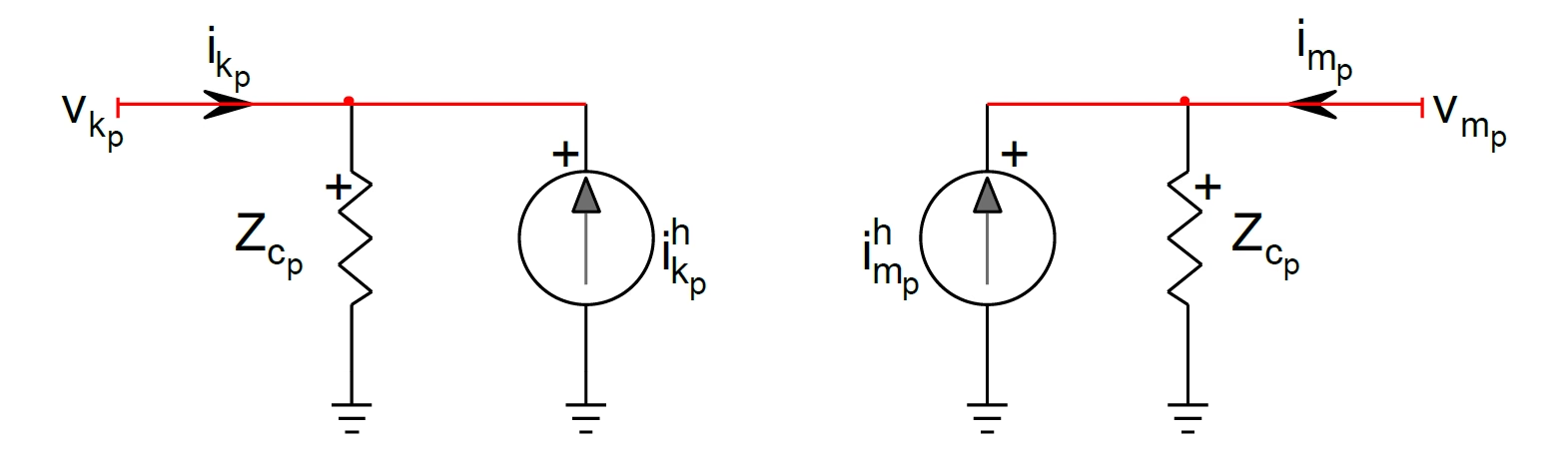
Each mode is realised as a lossless line with Norton-equivalent history sources at both ends — the classic Bergeron model. The transformation matrix is then used to return to the phase domain of the simulated network.

Lossless transmission-line model for one mode: at each end a characteristic impedance Z_cp in parallel with a history current source, linked by the propagation delay. — **Figure 2 —** Lossless travelling-wave model for one mode \(p\): each end has the characteristic impedance \(Z_{cp}\) in parallel with a history-term current source \(i^{\,h}\), coupled across the line by the propagation delay \(\tau_p\).

The losses are then re-introduced by distributing the modal series resistance around two lossless half-sections — one quarter of the resistance at each end and one half in the middle. This lumped-loss approximation is valid provided the resistance is small compared with the characteristic impedance, \(R'_p\ell\ll Z_{cp}\).

Complete CP model with losses: series resistance R'-ell/4 at each end and R'-ell/2 in the middle, between two lossless line halves of length ell/2. — **Figure 3 —** The complete CP model with losses — the modal resistance is lumped as \(R'_p\ell/4\) at each end and \(R'_p\ell/2\) in the centre, between two lossless half-lines of length \(\ell/2\).

When to use CP — and when not to

CP suits preliminary or narrow-band work: early screening of a large network, basic switching studies, training examples and sensitivity runs where speed matters more than precision and the system is reasonably balanced. It should not be the final model for lightning or very fast transients, GIS and high-frequency phenomena, long underground or submarine cables, HVDC cables, strongly unbalanced or untransposed systems, or insulation coordination with small margins. Always document the chosen model frequency, and benchmark against FD or WB for important cases.

Section 5

FD — Frequency Dependent model

Unlike CP, the FD model represents the frequency dependence of the line parameters. It still uses modal decomposition, so its accuracy hinges on whether the transformation matrix can be treated as real and constant — which is generally true for balanced or continuously transposed overhead lines, where FD is very accurate.

The transformation-matrix options

The exact transformation matrix \(T_i\) (the Q matrix) is complex, but FD cannot use a complex matrix. For a balanced line it uses the real, constant Clarke matrix. For an unbalanced line it offers two ways to obtain a real matrix:

Minimize Imaginary (the default): the exact complex transformation matrix is rotated so that its imaginary part is driven to zero.
Gmode = 0: the transformation is rotated so that the modal conductance — the real part of the shunt admittance — is driven to zero.

The two options are equivalent in most cases; the default can be used with confidence. Each modal characteristic admittance \(Y_c(s)\) and propagation function \(H(s)\) is then sampled over the frequency range and curve-fitted (a Bode-based technique) into rational functions:

\[ Y_c(s)\approx r_0+\sum_{i=1}^{N}\frac{r_i}{s-a_i} \qquad H(s)\approx\left(\sum_{i=1}^{M}\frac{c_i}{s-p_i}\right)e^{-s\tau} \]

\(r_i,\ c_i\): residues of the rational fits
\(a_i,\ p_i\): poles of the rational fits
\(r_0\): asymptotic (high-frequency) value of \(Y_c\)
\(\tau\): modal time delay extracted from \(H(s)\)

The fitted rational functions are discretised for time-domain integration, giving a delay-based model with history terms found by convolution. The FD model options are the Q-matrix type and frequency, the minimum scanning frequency \(f_\text{min}\), the number of points per decade, and the number of decades.

When to use FD — and when to be cautious

FD suits frequency-dependent overhead-line studies where the line is balanced or continuously transposed and full WB accuracy is not required — energisation, switching overvoltages, line-fault transients and travelling-wave studies. Be cautious, or prefer WB, for complex cable systems, multiple metallic layers, strongly unbalanced arrangements, very-high-frequency studies, submarine and HVDC cables, or whenever a stable, passive fitted model cannot be obtained.

Section 6

WB — Wideband model

The Wideband model is the most accurate model for time-domain simulation of lines and cables, and the recommended choice over a wide frequency band. It works directly in the phase domain and accounts for the full frequency dependence of the parameters — there are none of the modal-domain approximations of CP or FD. The characteristic admittance \(Y_c(s)\) and propagation function \(H(s)\) of the terminal equations are sampled over the chosen range and fitted by vector fitting:

\[ Y_c(s)\approx G_0+\sum_{i=1}^{N_y}\frac{G_i}{s-q_i} \qquad H(s)\approx\sum_{i=1}^{N}\left(\sum_{k=1}^{M_i}\frac{R_{i,k}}{s-p_{i,k}}\right)e^{-s\tau_i} \]

\(G_0\): constant matrix for \(s\to\infty\)
\(G_i,\ R_{i,k}\): matrices of residues
\(q_i,\ p_{i,k}\): fitting poles
\(\tau_i\): time delay of the \(i\)-th mode; \(N\) is the number of modes (conductors)

Vector fitting is a numerical method that replaces a complicated frequency response with a stable set of poles and residues. This is what lets EMTP® reproduce the frequency-dependent behaviour of a line or cable in the time domain — the residue matrices \(G_i\), \(R_{i,k}\) and the poles \(q_i\), \(p_{i,k}\) above are simply the result of that fit.

The time-domain solution again uses a delay-based circuit with Norton equivalents, but in the phase domain — so unbalanced systems and strong inter-conductor coupling are represented faithfully. The quality of a WB model depends strongly on the fitting controls.

Cable model correction (FDCM)

In coaxial cables with several conductors, conventional fitting can produce unbalanced modal contributions — high residue/pole pairs with opposite signs from different modal groups — which amplify integration errors and cause numerical instability. The cable model correction (FDCM) fits each modal contribution individually in the phase domain, avoiding these pairs and grouping repeated eigenvalues into smooth functions. The fitter switches to FDCM when the residue/pole ratio exceeds a threshold (default \(1000\)). More poles are needed than the conventional approach, but stability is greatly improved.

DC correction

HVDC simulations need the model to be precise close to DC, but extending the fitting band down to, say, below \(0.01\) Hz stiffens the fit. The DC correction feature partitions the frequency band to relax the fit and then adds a correction term for DC frequencies; it also helps maintain passivity. When DC correction is used, set the lower frequency limit \(f_\text{min}\) to \(0.001\) Hz or below. If the DC steady-state solution oscillates in the time domain, this option often resolves it.

Passivity — why it matters

A passive model cannot create energy by itself. If a fitted line or cable model is non-passive, the simulation may become unstable or produce artificial oscillations that do not exist in the real system. The WB procedure includes a passivity test; if violations occur, vary the fitting controls — convergence tolerance, frequency band, points per decade, grouping, DC correction or the advanced fitter — until the model is passive.

Fitting controls

Convergence tolerance — the target fitting error.
Cable model correction (FDCM) with its residue/pole threshold — for multi-conductor coaxial cables.
DC correction — for HVDC and near-DC accuracy.
Apply grouping — groups modes with near-identical delays; disabling it can sometimes correct stability.
Advanced fitter — optimises the time-delay calculation and the grouping criterion; recommended as an alternative when passivity is violated.
Scanning range — \(f_\text{min}\), points per decade and number of decades.

When to use WB

Use WB whenever accuracy matters: underground, submarine or pipe-type cables; mixed overhead-line/cable systems; lightning and very fast transients; GIS and high-frequency phenomena; HVDC cables (with DC correction); cases where sheath, screen or armour currents matter; unbalanced systems; wide frequency ranges; and insulation coordination with small margins. WB can also reproduce steady-state and frequency-scan behaviour accurately once properly fitted.

Section 7

Exact-PI and Nominal-PI models

Exact-PI

The Exact-PI model is a frequency-domain model used only for steady-state and frequency-scan simulations. It is an exact PI representation of the distributed line or cable as seen from its terminals, at each requested frequency. It must be calculated at the steady-state solution frequencies, and the frequency-scan range must match exactly the range selected for the model. WB can normally reproduce steady-state and frequency-scan results very accurately, so Exact-PI is provided chiefly for testing, referencing and benchmarking. Its series and shunt admittances follow directly from the terminal equations:

\[ Y_\text{series}=\frac{Y_c}{\sinh(\Gamma\ell)} \qquad\qquad Y_\text{shunt}=Y_c\,\tanh\!\left(\frac{\Gamma\ell}{2}\right) \]

\(Y_\text{series}\): series admittance of the equivalent PI
\(Y_\text{shunt}\): shunt admittance at each end of the equivalent PI
\(Y_c,\ \Gamma,\ \ell\): characteristic admittance, propagation constant and line length

Exact-PI is the right choice for harmonic-impedance scans, resonance identification, a frequency-domain reference solution, and validation of a WB model. It is not a time-domain model: it does not provide travelling-wave delays, and it cannot interact with nonlinear devices in the time domain.

Nominal-PI

The Nominal-PI model is a simple approximation: the per-unit-length parameters are calculated at a single frequency and multiplied by the length, giving a series impedance \(R+j\omega L\) and a shunt branch of \(C\) in parallel with \(G\), split between the two ends. It is fast and easy to interpret and suits fundamental-frequency studies, short lines and simple network equivalents — but it does not represent travelling-wave propagation or frequency dependence, so it should not be used for lightning, detailed switching, cable energisation or any high-frequency study.

Section 8

Choosing a model

Table 2 — Recommended model by study type.

Study	Recommended	Avoid as Final Model
Load flow / simple equivalent	Nominal-PI	—
Harmonic-impedance / frequency scan	Exact-PI (or validated WB)	Nominal-PI, CP
Line-energisation switching	FD or WB (lines); WB (cables)	Nominal-PI; CP as final
Cable energisation	WB	CP, Nominal-PI
Lightning overvoltage	WB (FD for OHL screening)	CP, Nominal-PI
Very fast transient / GIS	WB, high \(f\) range	CP, Nominal-PI
HVDC cable	WB + DC correction	CP, Nominal-PI, plain FD
Mixed OHL + cable	WB	One shared simplification

Modal domain versus phase domain

For overhead lines, modal-domain models (CP, FD) are often acceptable, especially when the line is balanced or transposed. For cables, phase-domain WB modelling is usually preferred, because cable systems are strongly coupled, geometrically complex and frequency dependent — exactly the conditions under which the real-transformation approximation of CP and FD is least reliable.

Section 9

Defining the conductor geometry

Before any model can be computed, the physical system must be defined on the Conductors tab. The main selection — overhead line, insulated cable, combined line and cable, or a per-unit-length parameter import — determines which data tables appear.

Overhead lines

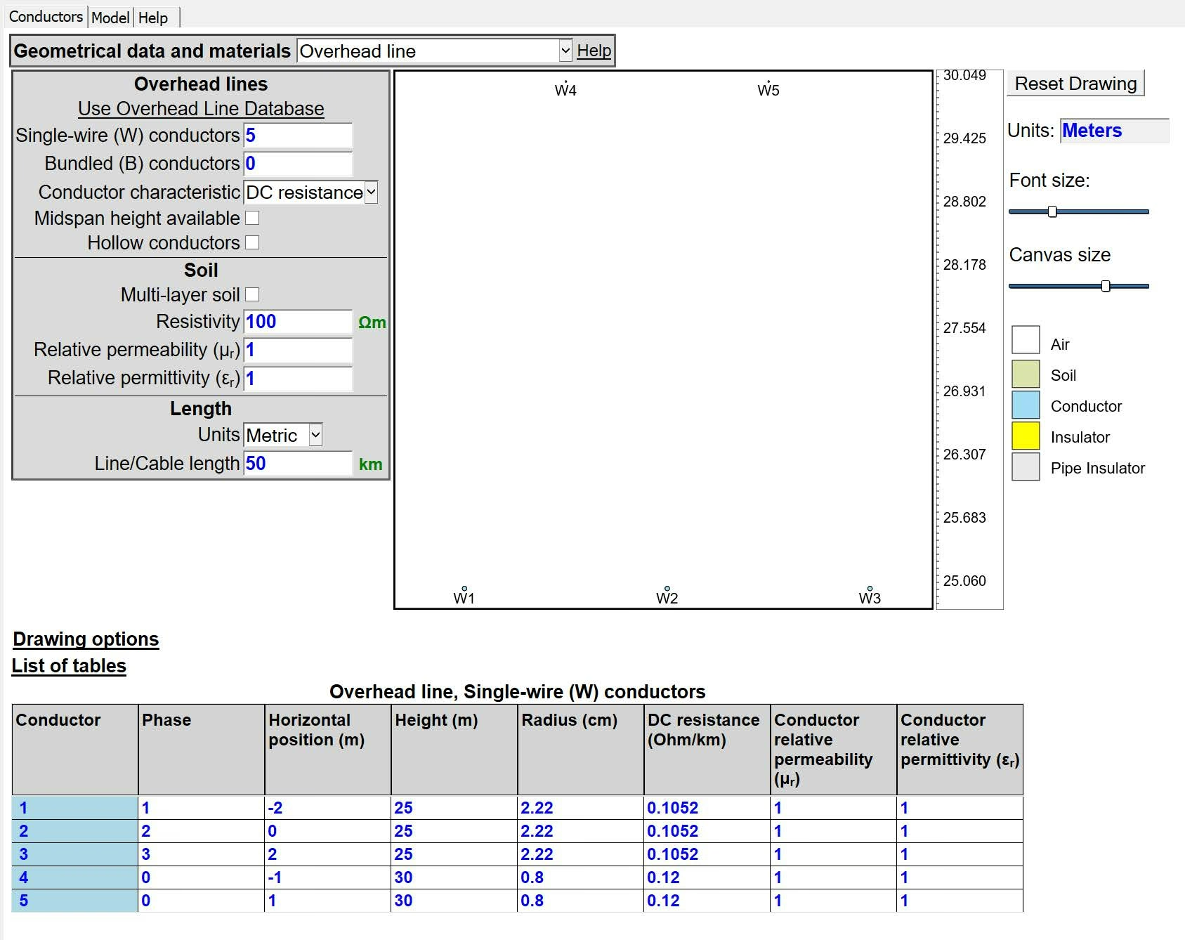
An overhead line is entered as single-wire and/or bundled conductors. The conductor characteristic can be given as a DC resistance or as a resistivity; a midspan height can be added where available; and tubular conductors are entered by checking the hollow-conductor option to expose an inner radius. After the number of conductors is set, a table is generated for the position and material properties of each one.

EMTP® Line/Cable Data device, Conductors tab, for a three-phase overhead line with two shield wires: geometry inputs, soil and length on the left, the cross-section drawing, and the single-wire conductor table below. — **Figure 4 —** The EMTP® **Line/Cable Data** device for a three-phase overhead line with two shield wires. Each conductor’s phase number, position, radius and resistance are entered in the table; a phase number of \(0\) reduces a conductor (e.g. a ground wire) out of the final model while still including its electromagnetic coupling.

In the Phase column, conductors are numbered from the top down. Assigning a phase of \(0\) makes a conductor inaccessible in the final model — the standard way to reduce ground wires so the model has only three pins per end, while still accounting for their coupling.

Bundled conductors

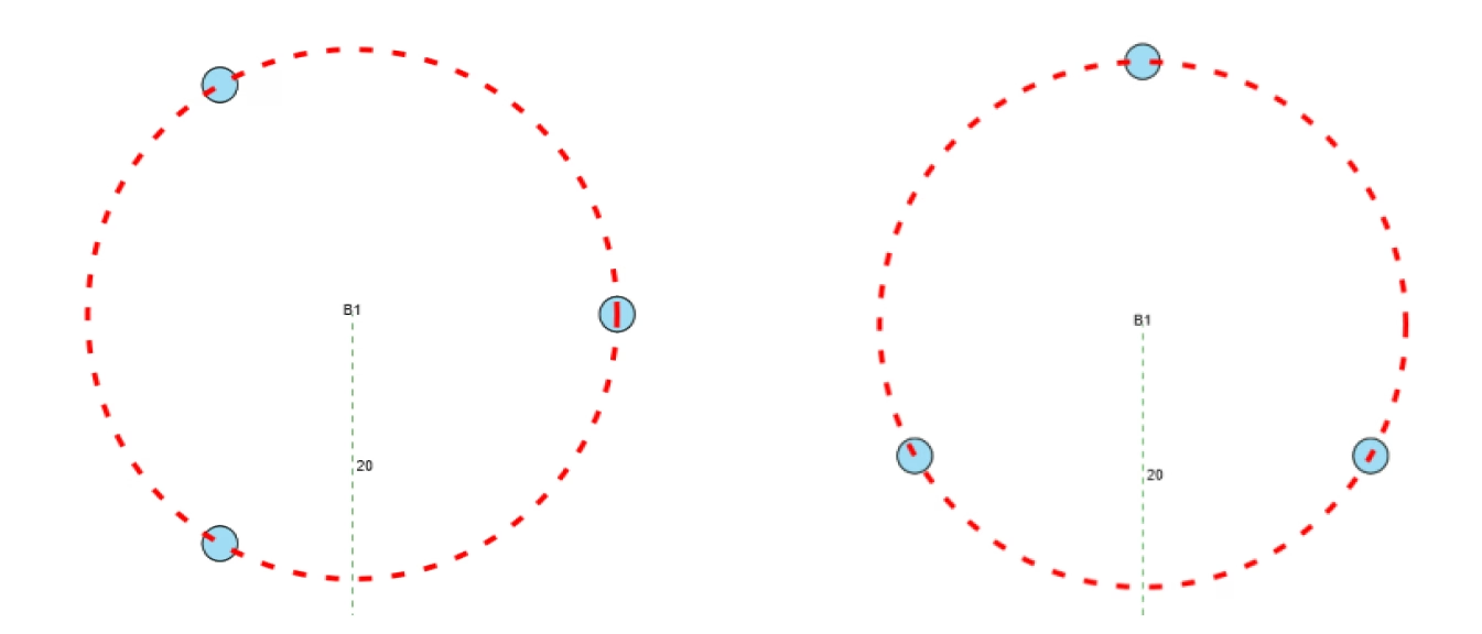
Modelling a bundle is equivalent to entering each subconductor individually and grouping them, but with far less data and only the phase pin exposed for connection. A bundle is defined by the number of subconductors, the bundle radius (or spacing), a reference angle and the conductor properties — all subconductors share the same radius and spacing. As a useful rule, the bundle radius of an equilateral triangle of three conductors is the side length divided by \(\sqrt{3}\).

A bundle of three subconductors shown at a 0 degree reference angle (left) and a 90 degree reference angle (right), arranged on a dashed bundle circle about the phase centre B1. — **Figure 5 —** A three-conductor bundle at a reference angle of \(0^\circ\) (left) and \(90^\circ\) (right). The reference angle orients the subconductors about the phase centre and can be set per bundle.

Predefined overhead-line configurations can also be loaded from the device’s built-in Overhead Line Database, then edited as needed.

Single-core cables

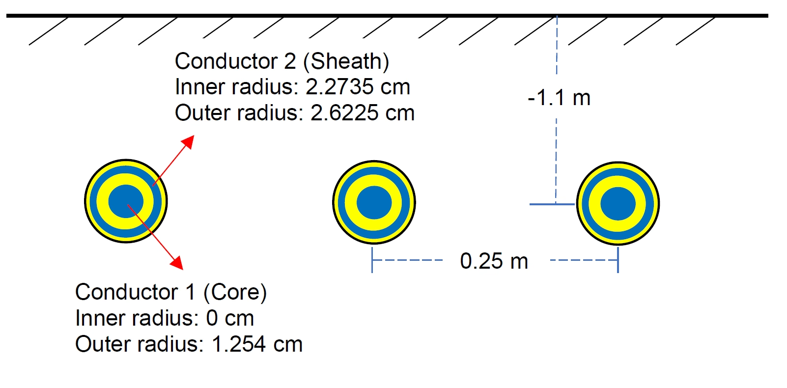
Insulated cables are entered as single-core coaxial cables or as pipe-type cables. A single-core cable needs both a main-data table and a conductor/insulator-layer table. A negative vertical position represents an underground cable; a positive value places it above ground.

Each conductor is assumed to be surrounded by an insulation layer, described by a relative permittivity and a loss factor \(\tan\delta\). The complex relative permittivity and its loss factor are:

\[ \varepsilon_r=\varepsilon_r'-j\,\varepsilon_r'' \qquad\qquad \tan\delta=\frac{\varepsilon_r''}{\varepsilon_r'} \]

\(\varepsilon_r',\ \varepsilon_r''\): real and imaginary parts of the relative permittivity
\(\tan\delta\): loss factor representing dielectric losses (the current penetrating the insulation)

Semiconducting layers

The thin semiconducting screens between a conductor and its insulation change the per-unit-length series impedance and shunt capacitance. The common practice is to absorb them into the surrounding insulation through an effective permittivity:

\[ \varepsilon_\text{new}=\varepsilon_r\,\frac{\ln\!\left(r_4/r_1\right)}{\ln\!\left(r_3/r_2\right)} \]

\(\varepsilon_\text{new}\): effective relative permittivity of the combined layer (insulation + semiconductor)
\(\varepsilon_r\): relative permittivity of the insulation material
\(r_1,\ r_2\): inner and outer radii of the semiconducting layer
\(r_3,\ r_4\): inner and outer radii of the insulation

The effective permittivity \(\varepsilon_\text{new}\) is entered in place of \(\varepsilon_r\). Alternatively, a semiconducting layer can be modelled explicitly as a further conductor with the appropriate resistivity.

Semiconducting screens are not a minor detail

For high-frequency cable transients, semiconducting screens should not be treated as a minor detail. If they are ignored or converted incorrectly, the model may give an unrealistically high propagation velocity and an incorrect surge impedance.

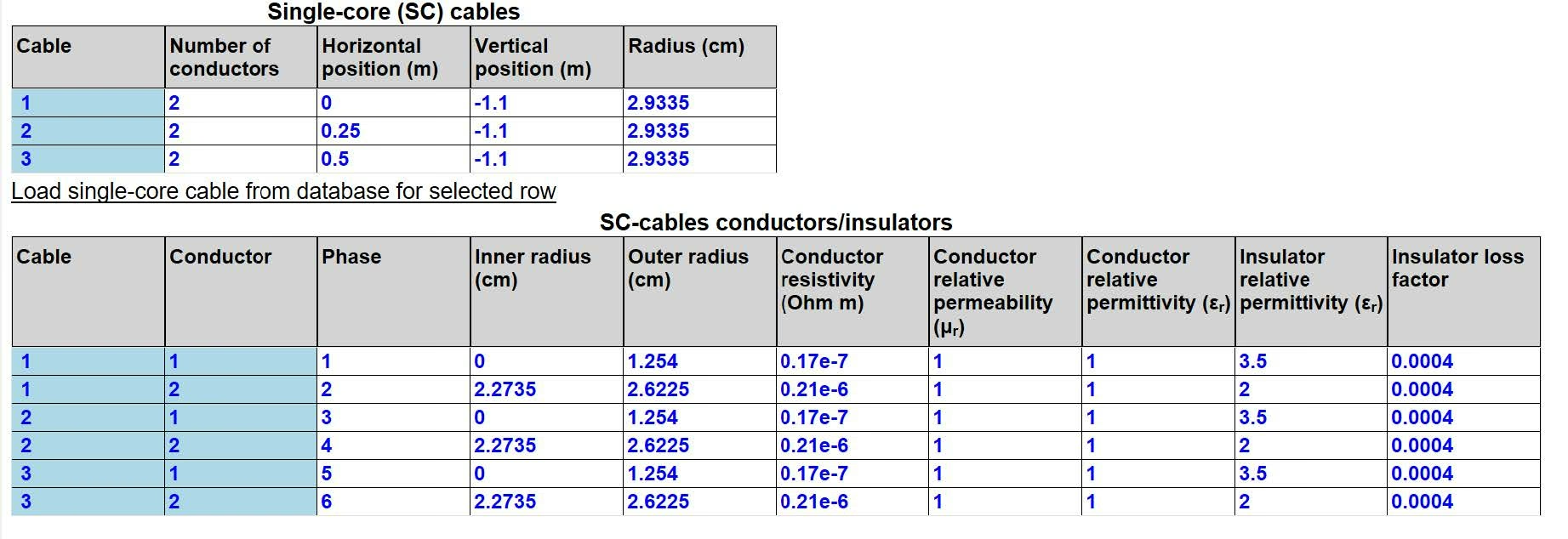
EMTP® Line/Cable Data device input for a three single-core cable system, showing the single-core main-data table and the conductor/insulator layer table. — **Figure 7 —** Entering the three single-core cable system of Figure 6 in the **Line/Cable Data** device — the single-core main data and the conductor/insulator layer data are entered in two linked tables. Predefined cables can also be loaded from the single-core cable database.

Pipe-type cables

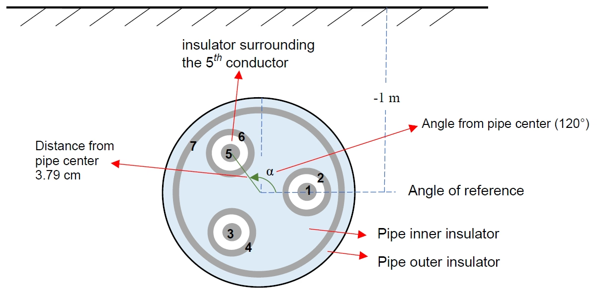
A pipe-type cable models several cores inside a common pipe or enclosure, with any number of coaxial layers per core; the same representation also covers tunnel-installed cables. It requires the position of each core relative to the pipe centre (a distance and an angle from the angle of reference), the pipe geometry, the insulation around the cores, the pipe insulation, the metallic layers and the cable depth.

A three-core pipe-type cable example: seven numbered conductors inside a pipe with inner and outer insulators, with the distance from the pipe centre, the angle of reference and a 120 degree angle marked. — **Figure 8 —** A three-core pipe-type cable. Each core is located by its distance from the pipe centre and an angle measured from the angle of reference; the conductor numbering feeds the **Phase** column in the data tables.

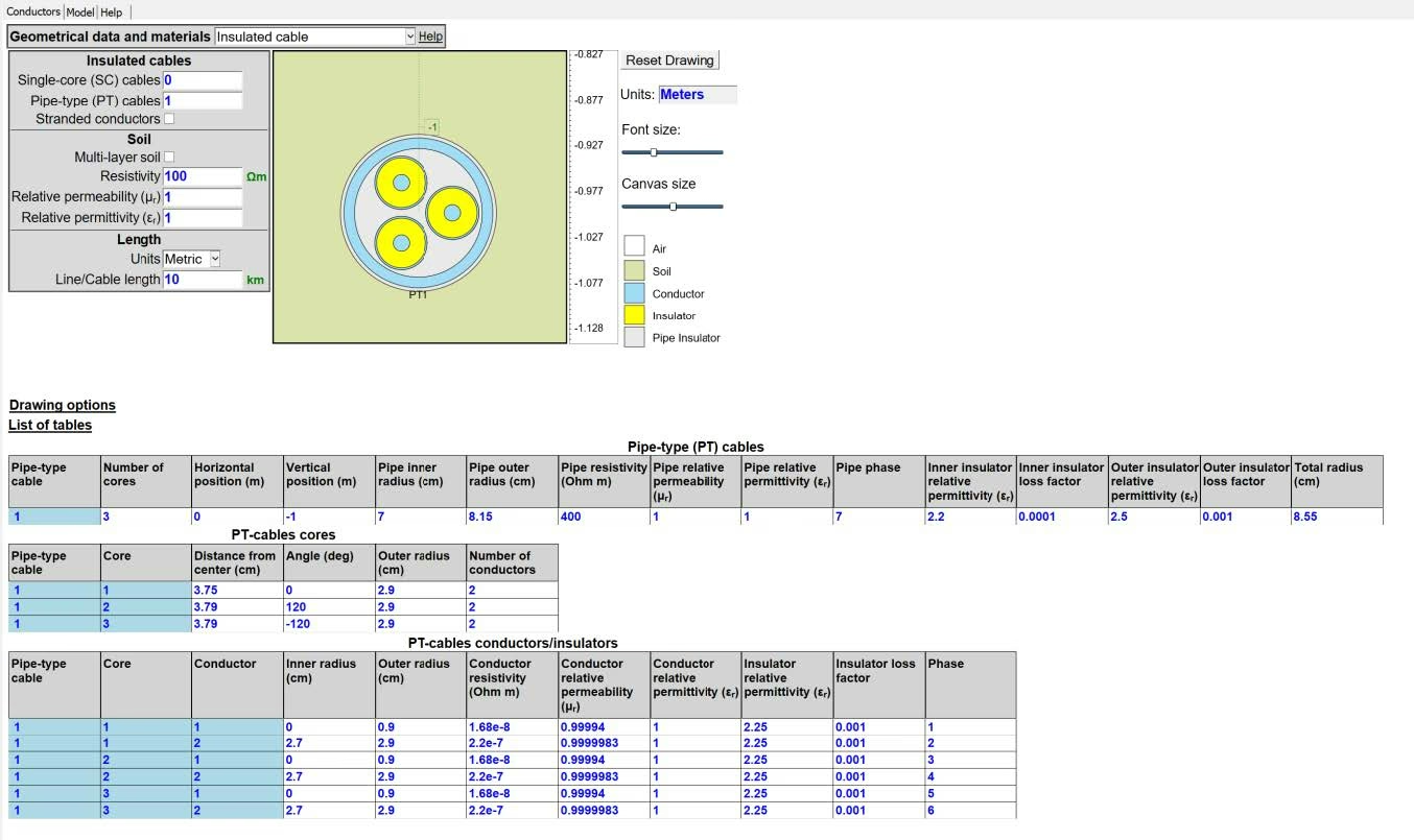
EMTP® Line/Cable Data device input for the pipe-type cable of Figure 8, with the pipe geometry and the per-conductor data tables. — **Figure 9 —** The **Line/Cable Data** device input for the pipe-type cable of Figure 8 — The *stranded conductors* option can represent a cylindrical conductor as a set of identical wires equally distributed over its surface, by entering the number of strands.

Importing per-unit-length parameters

Where the parameters are calculated externally, they can be imported from a MATLAB .mat file containing the variables Z, Y, f and line_length — the per-unit-length impedance and admittance matrices, the frequency vector and the length (no unit conversion is performed). The frequency vector is \(1\times N_\text{samples}\) and the matrices are \(N_\text{cond}\times N_\text{cond}\times N_\text{samples}\). CP needs a single frequency point; FD and WB need at least \(40\) logarithmically spaced samples; FD also needs the transformation-matrix frequency; and Exact-PI requires the samples to coincide with the frequency-scan frequencies.

Section 10

Soil modelling

The earth-return path affects both the impedance and the admittance, and the device offers a homogeneous or a multilayer soil model.

The homogeneous model uses one uniform resistivity and represents the earth-return path for both impedance and admittance. This return effect is important for high-frequency phenomena — GIS, lightning and surge analysis — where the propagation mode transitions (TEM to quasi-TEM, and quasi-TEM to full-wave) as frequency rises.

The multilayer model represents up to four soil layers and is important for submarine cables and stratified earth. Two practical rules apply: an underground cable should not be placed exactly on the boundary between two layers, and the deepest layer is treated internally as infinitely thick. The resistivity of the surrounding medium varies widely — wet soil is low, rock is high, and sea water is very low — so submarine-cable modelling should never assume the same return path as a land cable.

Section 11

Material properties and cable data

Cable modelling needs the resistivity and relative permeability of every conductor and the permittivity and loss factor of every insulation layer. Indicative values are given below.

Table 3 — Indicative conductor resistivities.

Material	Resistivity (\(\Omega\,\text{m}\))	Note
Copper	\(\approx 1.72\times10^{-8}\)	—
Aluminium	\(\approx 2.83\times10^{-8}\)	—
Lead	\(\approx 22\times10^{-8}\)	Common sheath material
Steel	\(\approx 18\times10^{-8}\)	Permeability \(\neq 1\) — armour, pipes

Table 4 — Indicative insulation relative permittivity.

Insulation	Relative Permittivity
XLPE	\(\approx 2.3\)
Mass-impregnated	\(\approx 4.2\)
Fluid-filled	\(\approx 3.5\)

Steel is more complex because its relative permeability is not unity and varies with magnetic condition — important for armour, pipes and magnetic enclosures. Stranded conductors are usually represented as an equivalent solid conductor, with the resistivity increased by the inverse of the surface fill factor so that the resistance is correct; without this correction the model under-estimates resistance and attenuation. Extruded insulation such as XLPE is practically lossless over a wide band, whereas paper-oil insulation can be appreciably lossy. Where a tool only accepts a constant loss factor and the real insulation is frequency dependent, it can be better to set the loss angle to zero than to impose an unrealistic constant \(\tan\delta\) across a very wide band. Semiconducting screens can have resistivity below \(10^{-3}\,\Omega\,\text{m}\) and relative permittivity above \(1000\); careless treatment distorts surge impedance and propagation velocity.

Section 12

Modelling options

Depending on the selected model, the device exposes several options that change what physics is represented.

Proximity effect — represents the non-uniform current distribution caused by nearby conductors; important for closely packed cables. Some older parameter routines include skin effect but neglect proximity effect, so always confirm whether the chosen routine and option actually include it.
Earth-return shunt admittance — accounts for the real part of the shunt admittance, which is not zero and becomes significant at high frequencies (about \(10\) kHz and above).
Enter G shunt — an artificial conductance to ground, used to model leakage through contaminated insulators. It is not a tuning factor and should only be used with a physical basis.
Balanced line — assumes a continuously transposed line; all mutual impedances and admittances are averaged.
Segmented ground wires — for ground wires grounded at one tower and insulated at adjacent towers; the mutual impedance between phase and ground wire is forced to zero.
Cross-bonded — for three identical single-core cables of two conductors each (core and sheath); the sheath impedances and admittances are averaged with no reduction (the cross-bonded conductors are identified by phase \(0\)).
Cross-bonded and reduced (the homogeneous model) — as above, but the sheath conductors are grouped into a single common conductor (the last conductor).
Twisting effects — for pipe-type cables with stranded wires; reduces the screen impedance terms to account for the three-dimensional twist of the cable.

Cross-bonding — when to keep it detailed

Cross-bonding divides the route into minor sections and transposes the sheaths so that the induced voltages tend to cancel over a major section (three minor sections), with grounding at the major-section ends. The averaged options are convenient, but do not use them when the circuits are not identical, when link boxes or sheath-voltage limiters are modelled, when sheath transients or individual sheath voltages are the objective, or when fault-current return through each sheath must be calculated accurately.

Section 13

Common mistakes, reporting and summary

Common modelling mistakes

Using Nominal-PI for transient studies — it cannot represent travelling-wave propagation.
Using CP for cables without validation — cables are strongly frequency dependent.
Ignoring sheath, screen or semiconducting layers, which often dominate cable behaviour.
Choosing a homogeneous soil model where stratified soil is important.
Setting a frequency range that excludes important transient content for FD or WB.
Ignoring passivity violations in a WB model.
Using the balanced-line assumption on a line that is significantly untransposed.
Over-simplifying cross-bonded cables when individual sheath voltages matter.
Modelling stranded conductors as solid without a fill-factor correction.
Ignoring armour or pipe effects during ground faults, where they dominate zero-sequence impedance.

What a model report should state

A defensible line or cable model should record:

the model purpose and the study it supports;
the physical system — type, voltage, circuits, conductors, length, installation, soil and bonding;
the input data — geometry, material properties, layer radii, permittivity, loss factor, soil resistivity and frequency range;
the selected model (CP, FD, WB, Exact-PI or Nominal-PI) and why it was chosen;
the model options — proximity effect, earth-return shunt admittance, cross-bonding, cable model correction, DC correction, fitting tolerance, points per decade and the passivity result;
for cables, how manufacturer data were converted — semiconducting layers, stranding, armour, pipe and dielectric-loss treatment, and whether each simplification is acceptable;
every assumption and limitation.

Key message

Choose the line or cable model from the physical phenomenon being studied, not from convenience. Use Nominal-PI for simple steady-state representation, CP only for preliminary or low-frequency transients, FD for frequency-dependent overhead lines where the modal assumptions hold, WB for accurate cable, overhead-line and mixed-system transients, and Exact-PI for frequency scans and benchmarking. Then document the assumptions, frequency range, soil model, conductor geometry, bonding and fitting options — because a cable’s real construction is always more complex than the idealised model, and the simplifications must be shown to be acceptable for the study objective.

Built on EMTP® · Expert spotlight

Henry Gras

Chief Operating Officer, PGSTech · Montréal, Canada

Henry is based in Montréal, where he is COO of PGSTech — the company responsible for the engineering services, commercialisation and continuing development of EMTP® (www.emtp.com). He holds a master’s degree from Polytechnique Montréal, where he spent two years on a research project on electrical machines, and previously completed an engineering degree at École Centrale de Lyon in France.

His technical expertise spans the simulation of power systems, electromagnetic transients, renewable energy, machines and protection. He and his team specialise in the full range of transient studies — from transient recovery voltage and renewable-energy integration to transformer energisation, ferroresonance, insulation coordination and power quality.

Beyond the engineering, Henry is genuinely kind and understanding, and consistently generous with his time — always willing to help others grow and to promote good technical work. If you would like to give EMTP® a try, or you need engineering services, he is a great person to reach out to.

Part 1 Reading now

Cable & Overhead Line Modelling

The model-family overview — choosing lumped, distributed or frequency-dependent line and cable models for the transient.

Series progress 1 of 16

Part 2

EMTP® Modelling of Insulated Power Cables

The cable-specific workflow — Cable Constants conversion, conductors, insulation, semiconducting screens, bonding and earth/sea return.