Renewable Modelling · EMT Models

EMT Models for Inverter-Based Generation

When the phenomenon lives outside the fundamental frequency — switching transients, harmonics, sub-synchronous interactions, a converter on a weak grid — an RMS phasor model runs out of road, and you reach for an electromagnetic-transient (EMT) tool such as EMTP®. This guide is about building inverter-based generation (IBG) models in that world: what EMT actually solves and why it is slow, the numerical trouble that ideal switches cause, the three levels of inverter detail and the ladder of controller models up to the manufacturer’s exact code, how to choose the right detail for a given study, and the AC-system strength that decides when EMT is not optional at all. It is the EMT companion to the model-selection guide and the detailed / average-value converter-model guides.

Reading time ≈ 36 min · Algorithm, detail levels, model selection & initialisation

The previous guide explained RMS / phasor modelling, where the fundamental-frequency behaviour of the network is represented by phasors — a magnitude and an angle. This guide explains EMT modelling, where the instantaneous voltages and currents are solved directly in the time domain, sample by sample. The central question here is the mirror of the last page: when is the RMS simplification no longer enough, and how much EMT detail does the study actually need? With both modelling methods now in hand, the guides that follow apply them study by study, beginning with frequency stability.

EMT and EMTP® — a quick definition

EMT stands for electromagnetic transient. An EMT simulation solves the instantaneous voltage and current waveforms in the time domain, rather than a magnitude and angle. EMTP® is one family of EMT simulation tools used for electromagnetic-transient and detailed converter studies. Keep the distinction in mind: EMT is a study method; EMTP® is a software environment in which that method is carried out (there are others).

Abbreviations used on this page

EMTElectromagnetic transient (time domain)

EMTP®Electromagnetic Transients Program (an EMT tool)

RMSRoot-mean-square (phasor) simulation

IBGInverter-based generation (or generator)

PVPhotovoltaic

WTGWind-turbine generator

DFIGDoubly-fed induction generator

VSCVoltage-source converter

MMCModular multilevel converter

HVDCHigh-voltage direct current

FACTSFlexible AC transmission systems

SVCStatic VAr compensator

STATCOMStatic synchronous compensator

IGBTInsulated-gate bipolar transistor

PLLPhase-locked loop

PWMPulse-width modulation

PIProportional–integral controller

SCRShort-circuit ratio

ESCREffective short-circuit ratio

PCCPoint of common coupling

DRTSDigital real-time simulator

FFT / DFTFast / discrete Fourier transform

FDNEFrequency-dependent network equivalent

NDANon-disclosure agreement

FRTFault ride-through

LVRT / HVRTLow- / high-voltage ride-through

SSR / SSTISub-synchronous resonance / torsional interaction

SSCISub-synchronous control interaction

Key idea

EMT solves the instantaneous three-phase waveforms in the time domain, so it sees what RMS hides — switching, dc components, unbalance, harmonics, travelling waves and fast control and protection. It is needed when the phenomenon is too fast, nonlinear, unbalanced or switching-dependent for RMS.
The Dommel method turns each dynamic element (inductor, capacitor, line) into a companion model — a resistor plus a history source — so every time step is a solvable algebraic circuit; ideal switches and the small time step dominate the numerical performance.
Model detail must match the study, in two separate axes: the electrical converter (simple-source → averaged-switch → discrete-switch) and the controller (generic → custom-detailed → exact compiled code).
Weak grids and the converter controls often decide whether EMT is essential: system strength (SCR / ESCR), a frequency-dependent network, and the protection logic frequently determine the answer — and a properly initialised model is a precondition for any of it being right.

Key terms used on this page

01EMT model

A three-phase, time-domain model that solves the network’s instantaneous waveforms and resolves fast transients.

02Companion model

The Dommel equivalent of a dynamic element: a resistor in parallel with a history current source, rebuilt each time step.

03History source

The current source in a companion model that carries the element’s stored energy forward from the previous step — its numerical memory.

04Sparse matrix

The network matrix, mostly zeros because each node connects to only a few others; solved efficiently with sparse techniques.

05Ideal switch

A switch modelled as an instant change between open and short circuit — convenient, but a source of numerical trouble.

06Bergeron line

A travelling-wave line model with a natural travel time and no direct end-to-end impedance; its delay lets subsystems decouple.

07Discrete-switch model

Every semiconductor device modelled individually with its gate pulses; the most accurate and the slowest.

08Averaged-switch model

The switching averaged into an equivalent source and impedance (\(E_{eq}\), \(R_{eq}\)); efficient, and the usual choice for an MMC.

09Simple-source model

The converter as a controlled voltage or current source; fast, for external-system studies, not for internal stress or harmonics.

10Black-box model

A vendor model whose internal logic cannot be inspected; protects intellectual property, but hides protection and limiter behaviour.

11SCR / ESCR

Short-circuit ratio and its effective form: the grid strength at the connection point relative to the converter rating.

12Initialisation

Settling the model to a consistent steady state before the disturbance, so it does not create artificial transients of its own.

Section 1

Why EMT, and what it captures

Two model families dominate power-system simulation, and the difference between them is the whole of this page. In an RMS simulation the waveform is simplified into a magnitude and an angle. In an EMT simulation the actual time-domain waveform is calculated sample by sample. That is why EMT can see switching pulses, unbalanced phase behaviour, travelling waves, harmonic content, dc-side behaviour, and fast controller and protection actions that RMS may hide.

Figure 1 — The same voltage disturbance, two ways. The RMS model (left) tracks the smooth voltage magnitude; the EMT model (right) resolves the instantaneous waveform, including the switching ripple and the distorted, asymmetric shape during the fault. RMS is far faster; EMT sees what RMS averages away.

Concretely, an EMT model can represent:

individual phase voltages and currents;
dc components;
unbalanced faults;
converter switching, and PWM effects if modelled;
fast PLL and current-control behaviour;
protection actions in a few milliseconds;
harmonic and sub-synchronous components;
transformer saturation and other nonlinear devices;
frequency-dependent lines, cables and transformers.

All of that comes at the price of speed. EMT follows the instantaneous waveform, so the time step must be small enough to capture the fastest event in the study. A 50 Hz waveform has a 20 ms cycle, but converter switching, protection operation and cable travelling waves may need steps down at the microsecond level — and the smaller the step, the more calculations per second of simulated time. That is the whole speed / accuracy trade-off in one sentence, and it is why EMT is reserved for the cases that need it. For where EMT sits against RMS on a weak grid, see EMT versus RMS on a weak grid.

Section 2

The Dommel method

How does a program solve a network of inductors, capacitors and lines at every microsecond? The classic answer is the Dommel algorithm, built on trapezoidal integration, and the idea is more approachable than it first looks.

An inductor or a capacitor cannot be solved like a plain resistor, because its current and voltage depend on the past — an inductor resists a change in current, a capacitor resists a change in voltage. The trapezoidal rule converts each such dynamic element into an equivalent resistor plus a history current source. The resistor represents the present-step relationship; the history source carries the memory of the previous time step. With every dynamic element replaced this way, the whole network becomes, at each step, an ordinary algebraic circuit that can be solved directly.

Figure 2 — The Dommel companion model. A dynamic element (inductor or capacitor) is replaced, at each time step, by an equivalent resistance \(R_{eq}\) in parallel with a history current source that carries the element’s stored energy forward. The equivalent is recalculated every step.

Two terms deserve to be spelled out. The history current source is the mathematical memory of the inductor or capacitor: it tells the next time step how much energy was stored in the element at the previous step. And the network solve at each step is a sparse linear solve: the network equations form a large matrix, but because each node connects to only a few others, most of the matrix entries are zero — a sparse matrix — and EMT programs use sparse-matrix techniques to solve it quickly every step. Transmission lines, transformers and machines are all derived the same companion way.

Why trapezoidal integration in particular? It is guaranteed numerically stable for linear circuits (higher-order rules can go unstable), and it is a second-order approximation between successive steps, so the smaller the step the more accurate the result. That accuracy limit is where the time-step rules of thumb come from.

What happens at each EMT time step

1. Update the switch, control and protection states.
2. Convert inductors, capacitors and lines into their companion models.
3. Assemble or update the network matrix.
4. Solve the node voltages and branch currents.
5. Update the stored-energy / history terms.
6. Pass the measurements to the controls and protection.
7. Move to the next time step.

On the time step itself, the rule of thumb is at least 20 time steps per cycle at the highest frequency of interest. Read it carefully: this is a minimum for representing a sinusoid reasonably, not a guarantee that 20 steps suffice for every study. For a 50 Hz fundamental, 20 steps per cycle is about 1 ms — but converter switching, lightning and surge studies, cable travelling waves and fast protection often need microsecond steps. Match the step to the fastest event you need to resolve, not to the fundamental.

Section 3

Modelling switches — the hard part

Power-electronic switches are where EMT gets difficult. An ideal switch changes instantly from an open circuit to a short circuit. That instant change is a sudden topology change in the network matrix, and it can create numerical oscillations, artificial voltage or current spikes, or convergence problems. Force an inductor current to zero in a single step \(\Delta t\) and you get an artificial voltage spike proportional to \(L\,i/\Delta t\) — the smaller the step, the bigger the spike. The physical device (an insulated-gate bipolar transistor, IGBT, for example), of course, has non-zero resistance, capacitance, inductance and a finite switching time, so perfectly ideal switching is a numerical convenience, not a physical truth.

The cures — and what each one does

Interpolation — estimates the exact switching instant between two time steps and corrects the solution to it, reducing the timing error and avoiding two devices switching in the same step.
Critical-damping adjustment (CDA) — damps the artificial high-frequency numerical oscillation that trapezoidal integration can show after a sudden change (for example a half-step of backward Euler).
Snubber circuits — small resistor–capacitor (or R–L–C) elements added around a switch to give the current and voltage a realistic path and improve numerical stability, much as real snubbers do in hardware.

When does the switching detail actually have to be there? Use a detailed switching model when the study depends on the harmonic spectrum, switching ripple, converter internal stress, electromagnetic interference (EMI), filter resonance, protection that uses the waveform shape, converter control interaction at switching or sub-synchronous frequencies, or validation against a manufacturer’s switching-level model. Use an averaged EMT model when the study needs the fast converter controls but not the individual switching pulses — which covers a great deal of dynamic and control-interaction work.

Section 4

Subsystems, real-time and hybrid simulation

Because EMT is slow, several techniques make large cases tractable. The first is subsystem splitting using travelling-wave lines. A distributed-parameter (Bergeron) line has a natural travel time: a disturbance at one end takes a real, finite time to reach the other. If that travel time is longer than the simulation time step, the two ends do not need to be solved simultaneously — the far end only reacts after the wave’s natural delay. That lets the network be split into smaller subsystems that can be solved separately, or on different processors, each at its own step. It is a numerical and computational advantage, not a different physical network — the delay is genuinely there in the real line.

That decoupling is the backbone of real-time digital simulation. A real-time simulator (a DRTS) must finish each calculation step before the next real-time step arrives: if the step is 50 µs, it has less than 50 µs to solve the network, run the controls, and handle its input/output. That is exactly why model simplification and subsystem splitting matter so much in real time.

Real time brings its own switch trick. Changing the network matrix every time a switch opens or closes can be too slow, so some methods keep the matrix structure constant and represent the switching by changing source terms or equivalent states instead. This is faster but introduces an approximation, and the chosen \(R\), \(L\) and \(C\) values control how accurate that approximation is. The guiding idea is to match the stored energies so the artificial switching loss is small: a capacitor stores \(\tfrac{1}{2}\,C v^2\) and an inductor stores \(\tfrac{1}{2}\,L i^2\), so choosing the values so that

\[ \tfrac{1}{2}\,C v^2 = \tfrac{1}{2}\,L i^2 \quad\Longleftrightarrow\quad C v^2 = L i^2 \]

In words: the capacitor’s stored energy depends on its voltage, the inductor’s on its current; matching the two stored energies minimises the artificial switching-loss error the fixed-matrix method would otherwise introduce.

Finally, hybrid EMT–RMS simulation runs the two methods together. The EMT part models the detailed converter or local network; the RMS part models the large surrounding power system; and the two exchange equivalent voltage, current and power information at their interface. This lets a detailed converter be studied without modelling the whole national grid in EMT. The bridge between them is a Fourier transform: an FFT/DFT extracts the fundamental-frequency phasor from the EMT waveform so it can be handed to the RMS side, while the RMS side supplies a network equivalent back to the EMT side.

Section 5

Confidentiality and black-boxing

Vendor EMT models are often built from the manufacturer’s real control code, so they contain confidential logic and are treated as highly sensitive — users typically sign a non-disclosure agreement (NDA). Black-boxing seals the control and/or electrical model into a single object whose internals cannot be inspected: it protects the intellectual property, and it is common for grid-connection studies. The user can run the model but cannot see all of its internal logic — and the real risk is that the engineer cannot easily verify hidden protection, limiters or mode changes, which are often exactly what decides a fault study.

The practical defence is documentation. Always request the model documentation, the model version, the intended study range, the known limitations, the required time step, the valid grid-strength range, and the validation evidence.

Black-box model checklist

Before using a black-box EMT model, confirm:

software version compatibility;
required simulation time step;
model initialisation method;
valid operating range;
supported fault types and control modes;
protection settings included;
ride-through behaviour and current-limit logic included;
known limitations;
validation against factory or site tests.

Section 6

Phenomena that require EMT

Read Table 1 as a model-selection guide. The left column is the physical phenomenon, the middle column explains what makes it difficult, and the right column shows the study types where EMT is normally required.

Table 1 — Phenomena and studies typically performed with EMT-type models (after CIGRE Table 4.1).
Phenomenon	What makes it difficult	Type of studies
Behaviour in response to large voltage deviations	Device protection against damage, fault ride-through capability, grid support	Short-term voltage stability; transient stability; provision of short-circuit current; low / high-voltage ride-through
Other phenomena and studies	Low- and high-frequency controller interaction	Controller interactions; switching transients; harmonic studies

The two rows are broad, so it helps to unpack the specific cases that push a study into EMT:

Large voltage deviations and FRT — the detailed low- and high-voltage ride-through (LVRT / HVRT) and recovery behaviour, especially near zero voltage.
Short-circuit current from IBGs — a converter’s fault current is set by its control and limits, not by a fixed internal impedance.
PLL behaviour during faults — angle errors that change the injected currents.
Weak-grid converter control interaction — the fast control–impedance interplay RMS can miss.
Harmonic and resonance studies — non-fundamental components and network resonances.
Switching transients — energisation, faults and clearing at the waveform level.
Protection and momentary cessation — logic that acts on the waveform in milliseconds.
Unbalanced faults with sequence-current control — per-phase behaviour beyond positive sequence.
HVDC, FACTS, SVC and STATCOM interaction — multiple fast converters and compensators in close proximity.
Sub-synchronous control interaction (SSCI) — the converter control interacting with a series-compensated network below fundamental frequency, the control-driven counterpart of classical sub-synchronous resonance (SSR).

The practical message: EMT is not required because a plant is renewable. EMT is required when the phenomenon is fast, nonlinear, unbalanced, switching-dependent, weak-grid-dependent, or protection-dependent.

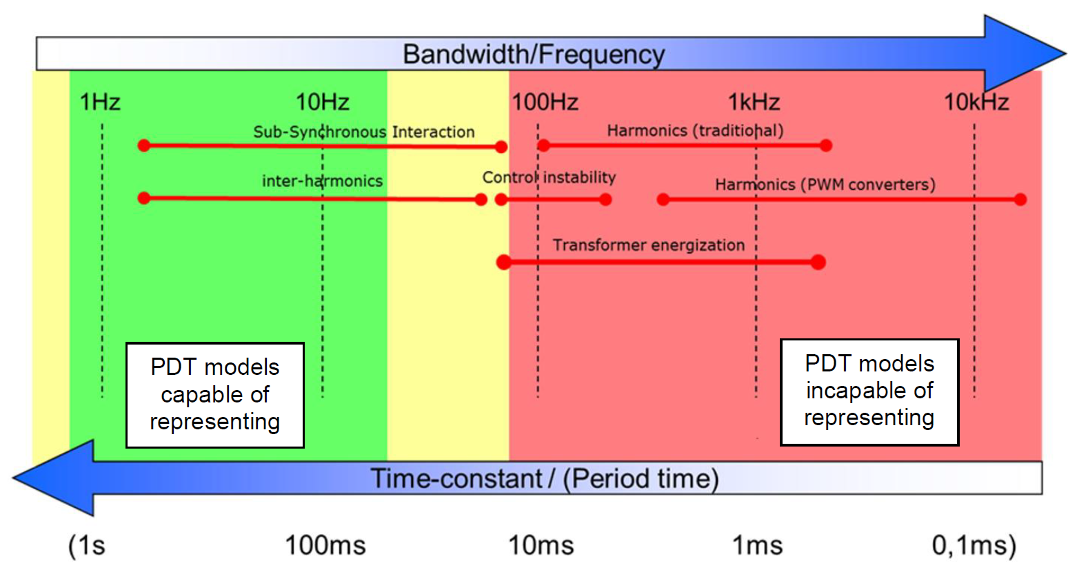
A single picture captures where the phasor model runs out of road. CIGRE’s brochure TB 881 places each phenomenon on a frequency axis and marks the band that a phasor-domain transient (PDT) model — what this series calls the RMS / phasor model — can and cannot represent (Figure 3). The rule of thumb it draws is simple: EMT tends to replace the phasor model once the phenomenon of interest has a dominant frequency more than about ±5 Hz from the fundamental, or once the system strength seen by the IBG falls near or below its withstand capability — the latter even when the dominant frequency sits at the fundamental. Everything in the red band — sub-synchronous interaction, control instability, traditional and PWM-converter harmonics, transformer energisation — is outside the phasor model’s reach.

Frequency-range chart from 1 Hz to 10 kHz with a matching time-constant axis. A green band up to roughly a few tens of hertz is labelled "PDT models capable of representing"; a red band from about 100 Hz to 10 kHz is labelled "PDT models incapable of representing". Red bars mark the frequency spans of sub-synchronous interaction and inter-harmonics (a few Hz to about 90 Hz), control instability (about 100 to 200 Hz), traditional harmonics and transformer energisation (about 100 Hz to 2 kHz), and PWM-converter harmonics (about 1 kHz to 10 kHz). — Figure 3 — Frequency range of power-system phenomena and the limits of phasor-domain transient (PDT) modelling. The phasor / RMS model covers the green band (up to roughly a few tens of hertz); sub-synchronous interaction, control instability, harmonics, PWM switching and transformer energisation fall in the red band, where EMT is required (after CIGRE TB 881, Figure 2.2-2).

Section 7

Inverter models, by level of detail

Here is a distinction that causes endless confusion, so it is worth stating first: an EMT model can be detailed in two separate ways — the electrical converter model and the control model — and the two must not be conflated. A model may pair a detailed controller with an averaged electrical converter, or a switching converter with a simplified controller. This section covers the electrical axis; the next covers the control axis, and Figure 4 shows both. The same electrical-detail choices apply whether the converter is the voltage-source converter (VSC) of a PV plant, a wind-turbine generator (WTG or DFIG), or an HVDC link.

Discrete-switch — every semiconductor device is represented explicitly, with its gate pulses, and the current paths change as switches open and close. It is the closest to the physical converter, and it is what you need for switching harmonics, converter stresses, detailed filter studies and some control-interaction studies. It is the slowest and needs detailed vendor data.
Averaged-switch — the switching is not followed pulse by pulse; the converter arm is replaced by an equivalent source and impedance representing the average effect of many switching events. This is especially useful for a modular multilevel converter (MMC), where modelling every submodule switch is impractical; it preserves the important converter dynamics while cutting the computation.
Simple-source — the converter is represented as a controlled voltage or current source; the internal switching and detailed arm behaviour are removed. It is useful when the external system response is the focus, and it is not suitable for internal converter stress, harmonics, or protection that reads the waveform shape.

Where the averaged-switch model collapses an arm, it does so as an equivalent circuit: an equivalent voltage source \(E_{eq}\) behind an equivalent resistance \(R_{eq}\). \(E_{eq}\) is the equivalent source that represents the converter arm (or a collapsed subnetwork) at that time step; \(R_{eq}\) is the equivalent resistance the network sees there; and both are recalculated as the converter’s internal state changes. They are numerical equivalents that reproduce the arm’s terminal behaviour — not physical components installed in the plant.

Figure 4 — The EMT model detail ladder. The electrical converter model (simple-source → averaged-switch → discrete-switch) and the control model (generic → custom-detailed → exact compiled code) are separate choices: a study may need a detailed controller with an averaged converter, or the reverse.

Section 8

Controller models, from generic to exact

The control axis runs in parallel with the electrical one:

Generic controller — standard blocks with approximate behaviour, useful for early screening and system-level studies.
Custom-detailed controller — project-specific logic built in the simulation tool, including the actual settings, limiters and protection.
Exact / compiled controller — the manufacturer’s control code, or a close compiled implementation of it, normally used for grid-code compliance and detailed EMT studies.

A caution on the word “exact”: it does not mean error-free. An exact model still has a valid operating range, a version, a parameter set and interface assumptions, and it must be used within them. On the standards side, IEC 61400-27-1 provides generic electrical simulation models for wind power generation; it is useful for standardised RMS-type model structures, but it does not replace a project-specific EMT vendor model where detailed converter behaviour is required — IEC 61400-27-1 alone is not enough for every EMT study.

Section 9

Choosing the detail for the study

The detail needed — in both the control model and the electrical model — follows the study. The end user should understand the phenomenon, know where the model approximates (what is included and what is not), and decide whether those approximations matter: a model missing some protection may be fine for a feasibility study but wrong for a final design. Table 2 maps common study types onto the control and electrical detail they call for.

Table 2 — Control-model and electrical-model detail by study type (after CIGRE Table 4.2).
Study	Control model required	Electrical model required
Feasibility study	All control models suitable	All models suitable
Transient over-voltages	Standard or custom-detailed, or exact	Interface (satisfactory), averaged-switch (better), discrete-switch (best)
Harmonics	All, if they represent the converter impedance at the harmonics of interest	Averaged-switch (satisfactory) or discrete-switch (best)
Interconnection study	Standard or custom-detailed (satisfactory), or exact (best)	Averaged-switch (satisfactory) or discrete-switch (best)
Weak-system studies	Standard or custom-detailed (satisfactory), or exact (best)	Averaged-switch (satisfactory) or discrete-switch (best)
SSTI / SSCI	Standard or custom-detailed (maybe), or exact (best)	Averaged-switch (satisfactory) or discrete-switch (best)
Control design & rating (by manufacturer)	Standard or custom-detailed (maybe), or exact (best)	Averaged-switch (satisfactory) or discrete-switch (best)
Interaction study	Standard or custom-detailed (maybe), or exact (best)	Discrete-switch

A quick model-selection guide (study objective → EMT detail)

Harmonic spectrum → discrete-switch, or a validated harmonic model.
Weak-grid control interaction → a detailed controller, often with an averaged or switching EMT converter.
LVRT compliance → a vendor EMT model with the FRT and protection logic.
Short-circuit current contribution → an EMT model with the current limit, PLL and protection.
MMC-HVDC dynamics → an averaged-switch or detailed MMC model.
Protection waveform study → a switching or sufficiently detailed waveform model.
Large-system screening → RMS first, with an EMT benchmark for the critical cases.

Section 10

The inner loop, the PLL, PWM and protection

EMT models often carry the controls that RMS models skip, so it is worth naming them in order. The PLL estimates the grid-voltage angle. The current controller calculates the voltage or current command needed to make the inverter track its active- and reactive-current references — usually a cascaded PI (proportional–integral) controller, whose proportional part reacts to the present error while its integral part removes the steady-state error over time. PWM then converts that command into gate pulses in a switching model; in an averaged model, PWM is represented by an average modulation signal rather than individual pulses. This is exactly the control chain introduced back in the inverter-characteristics guide, now solved at the waveform level. RMS programs usually skip the inner loop and inject the current references directly, which is precisely why RMS cannot see SSCI.

Internal protection often decides the answer

It is tempting to treat protection as an afterthought, but internal protection is often the part that decides the simulation result during a severe fault. It can limit current, block the pulses, enter momentary cessation, trip the converter, or change operating mode. If the study is about LVRT, short-circuit current or post-fault recovery, the protection logic cannot be ignored — and it is exactly the part a black-box model may hide. EMT measurements also have genuine delays (true-RMS or FFT/DFT), and effects such as a dc offset or a second harmonic during unbalance can be amplified by the measurement algorithm — realistic behaviour that simpler models smooth away.

Section 11

The ac system and its strength

The converter is only half the model; the surrounding ac system deserves the same care. The key indicator is system strength — the short-circuit MVA relative to the converter rating, the short-circuit ratio (SCR). Its effective form (ESCR) subtracts the reactive power of nearby shunt capacitors and ac filters, which weaken the fundamental-frequency impedance without adding short-circuit MVA:

\[ \mathrm{SCR} = \frac{S_{CMVA}}{P_n}, \qquad \mathrm{ESCR} = \frac{S_{CMVA} - Q_C}{P_n} \]

\(S_{CMVA}\): short-circuit power of the ac grid at the PCC (MVA)
\(P_n\): nominal power of the IBG (MW)
\(Q_C\): reactive effect of the IBG’s AC-side equipment — filters, shunt capacitors, synchronous condensers (Mvar)

A high SCR means a strong grid; a low SCR means the converter current has a large effect on the voltage angle and magnitude, so the PLL and current-control interactions become far more important.

As a rule of thumb, a weak system — SCR below about 5 — is where EMT tends to become essential. Treat that as a practical warning threshold, not a universal law: the model actually required depends on the converter control bandwidth, the PLL design, the grid impedance angle, nearby converters, filters, compensation and the operating condition. For very weak grids, vendor EMT models or impedance-based studies are normally required, and even a higher SCR can still pose problems.

One more piece of the ac system is easy to underrate. In an EMT study the surrounding network should not always be represented by a simple Thévenin impedance. Lines, cables, transformers, filters and loads may need a frequency-dependent representation — a frequency-dependent network equivalent (FDNE) for the far system, frequency-dependent line and cable models, transformer saturation, and proper resistor–inductor–capacitor filter models with their tuned resonances — whenever the study involves resonance, harmonics, switching transients or sub-synchronous interaction. The usual method is to build a large model and shrink it until the frequency response starts to degrade, or grow a small one until adding more stops changing the result.

Section 12

Model initialisation

An EMT model can be technically correct and still give wrong results if it is not initialised properly. Because EMT starts from instantaneous values, the model must be settled to a consistent steady state before the disturbance, or it will generate artificial transients of its own that contaminate the event you actually wanted to study.

The load-flow / steady-state starting point must match the intended operating point.
The controller states must be settled before the disturbance is applied.
The dc-link voltage, PLL angle, current references and plant-controller outputs must all be mutually consistent.
Otherwise the model may create artificial transients before the real event even begins.

Getting an inverter model to a clean flat start is a subject in its own right; see the dedicated guide on EMT initialisation and flat start.

Section 13

Common mistakes

The traps that most often catch an EMT IBG study — each one a theme from the sections above:

Eight traps to avoid

Using EMT with too large a time step for the fastest event in the study.
Using switching detail when an averaged model would do — paying for accuracy the study does not need.
Using a black-box model without checking its limitations, version and valid range.
Assuming a generic controller is valid for weak-grid interaction.
Ignoring protection or momentary cessation, so a plant that would trip is modelled as riding through.
Modelling the converter in detail but using an unrealistic grid equivalent (a bare Thévenin where a frequency-dependent network is needed).
Trusting EMT results before checking initialisation.
Confusing electrical converter detail with controller detail — the two axes of Figure 4.

Key points

EMT is not automatically better than RMS — it is more detailed and more expensive

Use EMT when the answer depends on instantaneous waveforms, switching, nonlinear devices, unbalance, fast controls, protection operation, weak-grid behaviour, harmonics or sub-synchronous interaction — then choose the simplest EMT model that still contains the converter, controller, protection and network detail the phenomenon needs. EMT solves the three-phase waveforms in the time domain by turning every dynamic element into a companion model (a resistor plus a history source), at a step matched to the fastest event, with ideal switching as the main numerical hazard that interpolation, the critical-damping adjustment and snubbers tame, and with subsystems, real-time and hybrid techniques keeping it tractable. Match the electrical detail (simple-source → averaged-switch → discrete-switch) and the controller detail (generic → custom-detailed → exact) to the study; keep the protection and measurement delays that make a real device trip; model the AC-system strength (SCR / ESCR) and its frequency response; and initialise before you trust anything. For where EMT sits against RMS and how the two compare, see the RMS-models guide, RMS versus EMT model selection, EMT versus RMS on a weak grid, and EMT initialisation and flat start.

References

The CIGRE/CIRED joint working-group brochure on inverter-based generation is the primary reference; Dommel’s 1969 paper is the origin of the EMT algorithm; IEC 61400-27-1 is the interfacing standard for wind-turbine models; and the EMTP® documentation is the reference for the tool itself.

CIGRE/CIRED Joint Working Group, Modelling of Inverter-Based Generation for Power System Dynamic Studies. CIGRE Technical Brochure.
H. W. Dommel, “Digital Computer Solution of Electromagnetic Transients in Single- and Multiphase Networks,” IEEE Transactions on Power Apparatus and Systems, vol. PAS-88, no. 4, pp. 388–399, 1969.
IEC 61400-27-1, Wind Energy Generation Systems — Part 27-1: Electrical Simulation Models. International Electrotechnical Commission.
EMTP®, Electromagnetic Transients Program — Documentation and Renewable / Converter Model Notes. Powersys / EMTP®.

Part 4 Reading now

EMT Models for Inverter-Based Generation

Electromagnetic-transient modelling: the Dommel method, switching, inverter detail levels and system strength.

Series progress 4 of 12

Part 5

Model Adequacy for Wide-Area EMT Studies

When a generic EMT model is adequate and when only a vendor-specific, site-specific model will do — the adequacy question for wide-area studies.