Test Procedures · Parameter Determination

Test Procedures for Synchronous Machine Parameter Determination

The accuracy of a synchronous-machine EMTP® model depends directly on the quality of its parameters — and those parameters come from tests. The purpose of testing is not to produce a list of numbers, but to identify the machine’s electrical and magnetic behaviour so it can be represented correctly. No single test gives everything: a good model combines data from several test families and then converts the measured characteristic quantities into the fundamental equivalent-circuit parameters. This guide covers the main test families — steady-state, sudden short-circuit, decrement, standstill frequency response and online — what each reveals, and how the data connects to the model.

Reading time ≈ 38 min · Steady-state, short-circuit, SSFR & online tests

A synchronous machine contains stator windings, a field winding, damper circuits, magnetic saturation, rotor inertia and mechanical coupling, and different tests reveal different parts of that behaviour. The model is normally built by combining several tests and then converting the measured characteristic parameters into the fundamental equivalent-circuit parameters the program needs.

Abbreviations used on this page

EMTP®Electromagnetic Transients Program

OCC / SCCOpen- / short-circuit characteristic

SSFRStandstill frequency response

AC / DCAlternating / direct current

RMSRoot mean square

\(L_d(s),\ L_q(s)\)d- and q-axis operational inductances

\(G(s)\)Armature-to-field transfer function

\(T_a\)Armature (DC-offset) time constant

\(X_d, X_q\)d- and q-axis synchronous reactance

\(X'_d, X''_d\)d-axis transient / subtransient reactance

SCRShort-circuit ratio

Key idea

Distinguish three things: the test procedure, the characteristic parameter it yields (e.g. \(X''_d\), \(T'_d\)), and the equivalent-circuit parameter the model needs — the last requires conversion.
No single test gives everything: steady-state tests give saturation and synchronous impedance, short-circuit/decrement tests give transient and subtransient data, SSFR gives operational inductances.
q-axis data is harder to obtain (no field winding) and is often less certain — the model should reflect that limitation.
A model is not complete until it reproduces the relevant measured response — not merely because it runs.

Key terms used on this page

01Test procedure

The physical test performed (OCC, SCC, slip, sudden SC, SSFR…).

02Characteristic parameter

A value derived from a test, e.g. \(X'_d\), \(T''_d\), the OCC.

03Equivalent-circuit parameter

An internal R or L the EMTP® model needs; obtained by conversion.

04Open-circuit characteristic

No-load voltage vs field current; saturation and air-gap line.

05Sudden short-circuit test

Fault applied to an open-circuited running machine; gives \(X'_d, X''_d, T'_d, T''_d\).

06Decrement test

Parameters from voltage/current decay after a switching action; open-circuit time constants.

07SSFR

Standstill frequency response; operational inductances and transfer functions over frequency.

08Operational inductance

\(L_d(s)\), \(L_q(s)\): effective inductance as a function of frequency.

09Slip test

Low-slip test estimating the q-axis synchronous reactance.

10Online test

Measurement while the machine runs connected; validation under operating conditions.

Section 1

Three concepts to keep separate

Parameter determination is central to machine modelling, and three ideas must be distinguished. A test procedure is the physical test performed — open-circuit, short-circuit, slip, voltage recovery, SSFR. A characteristic parameter is a value derived from a test — \(X_d\), \(X'_d\), \(X''_d\), \(T'_d\), \(T''_d\), \(X_q\), the OCC or the SCC. An equivalent-circuit parameter is the internal quantity the EMTP® model needs — stator leakage inductance, field resistance, damper resistance, field and damper leakage inductances and mutual air-gap inductance. Standards define how the tests are performed and how characteristic parameters are determined, but the final conversion into a specific equivalent circuit is still a modelling task that requires judgement.

Section 2

Why testing is needed before EMTP® modelling

EMTP® represents the machine by differential equations that need internal parameters — stator resistance and leakage, d- and q-axis mutual inductances, field resistance and leakage, damper resistances and leakages, and any field-damper leakage path. These are not measured directly. Tests excite, short-circuit, disconnect or perturb the machine and record the voltage, current, speed, field voltage or field current; characteristic quantities are then extracted from the waveforms. The engineer’s role is to convert those into a model that reproduces the measured response over the relevant frequency and time range. A machine model should therefore never be a black box — the test data, conversion assumptions and model structure must be consistent.

Section 3

Classification of machine tests

Acceptance tests

Verify contractual or manufacturing requirements — insulation, winding resistance, temperature rise, mechanical and vibration checks, performance verification. Important for acceptance, but not always sufficient for detailed transient modelling.

Performance tests

Determine operating characteristics — losses, efficiency, the OCC, the SCC, thermal performance. Some provide very useful modelling data: the OCC is essential for saturation, the SCC for synchronous impedance and SCR.

Parameter-estimation tests

Aimed specifically at deriving model parameters — sudden short-circuit, voltage recovery, load rejection, slip, SSFR and online disturbance tests. The most complete model normally needs both steady-state performance tests and parameter-estimation tests.

Section 4

Steady-state tests

Steady-state tests determine behaviour under slowly varying conditions. They do not directly give every transient parameter, but they provide essential base information: the open-circuit characteristic, the short-circuit characteristic, the d-axis synchronous impedance, the slip test for q-axis synchronous impedance, negative- and zero-sequence tests, and resistance measurements. For EMTP® modelling the most important are the OCC, the SCC and the slip test.

Section 5

Open-circuit characteristic test

The OCC is run at rated speed with the stator open and the field excited: the field current is varied and the terminal voltage (and shaft speed) recorded. It gives the relationship between field current and no-load terminal voltage; with the stator open the stator current is zero, so the voltage is mainly the d-axis air-gap flux produced by the field. At low excitation the OCC is nearly linear — that lower portion is extended to form the air-gap line — and at higher excitation it bends away as the iron saturates. The detailed air-gap-line and saturation-curve treatment belongs to the magnetic-saturation page; here the OCC is treated simply as a test output.

The OCC is the foundation of saturation modelling, air-gap line determination, unsaturated and saturated synchronous reactance, the short-circuit ratio, field-current-base checking, excitation-model validation and no-load voltage verification. A good test includes points below the linear region, several near rated voltage (the most important range), and some above where permitted. A frequent error is to enter a generic or incorrectly scaled OCC — producing realistic-looking waveforms but wrong field current, voltage recovery and load-rejection behaviour.

Section 6

Short-circuit characteristic and d-axis synchronous impedance

The SCC is run at rated speed with the stator shorted and the field excited: the field current is increased and the armature current recorded. It is normally almost linear up to rated current because the machine runs at low flux under short circuit. The key value is \(I_{fSC}\), the field current for rated armature current, compared with the field current for rated voltage on the OCC or air-gap line:

\[ X_{du} = \frac{I_{fSC}}{I_{fNL(ag)}} \qquad\qquad X_{ds} = \frac{I_{fSC}}{I_{fNL}} \]

\(X_{du},\ X_{ds}\): unsaturated and saturated d-axis synchronous reactance (pu)
\(I_{fSC}\): field current for rated armature current (SCC)
\(I_{fNL(ag)},\ I_{fNL}\): field currents for rated no-load voltage on the air-gap line and the actual OCC

The saturated value is normally lower, because the actual OCC needs more field current at rated voltage than the air-gap line. The synchronous reactance separates into an unsaturable leakage component \(X_l\) and a saturable mutual component (unsaturated \(X_{adu}\), saturated \(X_{ads}\)), so \(X_{du} = X_l + X_{adu}\) and \(X_{ds} = X_l + X_{ads}\) — useful because saturation is applied to the mutual path, not the leakage. The leakage reactance must therefore be treated carefully, since it affects the conversion and the leakage/mutual flux split.

Section 7

Slip test and why q-axis data is harder

The slip test estimates the q-axis synchronous reactance. The rotor is driven at a speed very close to synchronous with the field open, and the stator is fed from a balanced three-phase source below the saturation region. As the rotor slips slowly relative to the stator field, the field aligns first with the d-axis then the q-axis, and the measured voltage/current ratio varies between d- and q-axis values: aligned with the direct axis it corresponds to the d-axis impedance, aligned with the quadrature axis to the q-axis. A more accurate route takes \(X_d\) from OCC/SCC and then computes \(X_q\) from the slip-test ratios. The slip must be very small — too high a slip distorts the derived ratios. The result is approximate and sensitive to test conditions; for modern large machines, saturation and rotor eddy-current effects can reduce its accuracy, so the slip-test \(X_q\) is best treated as indicative.

q-axis parameters are intrinsically harder to obtain because there is no field winding on the q-axis; its behaviour is set by dampers, rotor geometry and solid-rotor current paths. Standard no-load sudden short-circuit tests give incomplete q-axis transient/subtransient data because the initial q-axis flux is zero at no load. Special procedures are needed, often complex and less common — so for EMTP® modelling, q-axis data may be uncertain, and the model should reflect that.

Section 8

Sudden short-circuit tests

A sudden three-phase short circuit applied to the initially open-circuited stator of a machine running at rated speed gives \(X'_d\), \(X''_d\), \(T'_d\) and \(T''_d\). The full physics of the subtransient, transient and steady-state decay is set out on the parameters and short-circuit response page; here the focus is how the test data is obtained and fitted. The field voltage must be held constant, because the analysis assumes constant excitation. The test is severe — high electrical and mechanical stress — so the number of tests is limited and they may be done at reduced voltage and extrapolated. Immediately after the fault the stator current contains a fundamental-frequency AC component and a DC offset; the AC component gives the reactances and time constants, the DC component gives the armature time constant. The AC rms current decomposes as:

\[ I(t) = I_{ss} + I'(t) + I''(t) \]

\(I(t)\): AC RMS short-circuit current envelope at time \(t\)
\(I_{ss}\): steady-state AC component, set by the d-axis synchronous reactance \(X_d\)
\(I'(t)\): transient decaying component, set by the d-axis transient reactance \(X'_d\) and transient short-circuit time constant \(T'_d\)
\(I''(t)\): subtransient decaying component, set by the d-axis subtransient reactance \(X''_d\) and subtransient short-circuit time constant \(T''_d\)

State the test conditions before using the parameters

Several sudden-short-circuit tests may be performed at different pre-fault open-circuit voltage levels. The selected test level affects the degree of saturation and the current duty. Therefore, the pre-fault voltage, saturation basis, RMS/peak convention, field condition and data-acquisition quality should be stated before the extracted parameters are used in EMTP®.

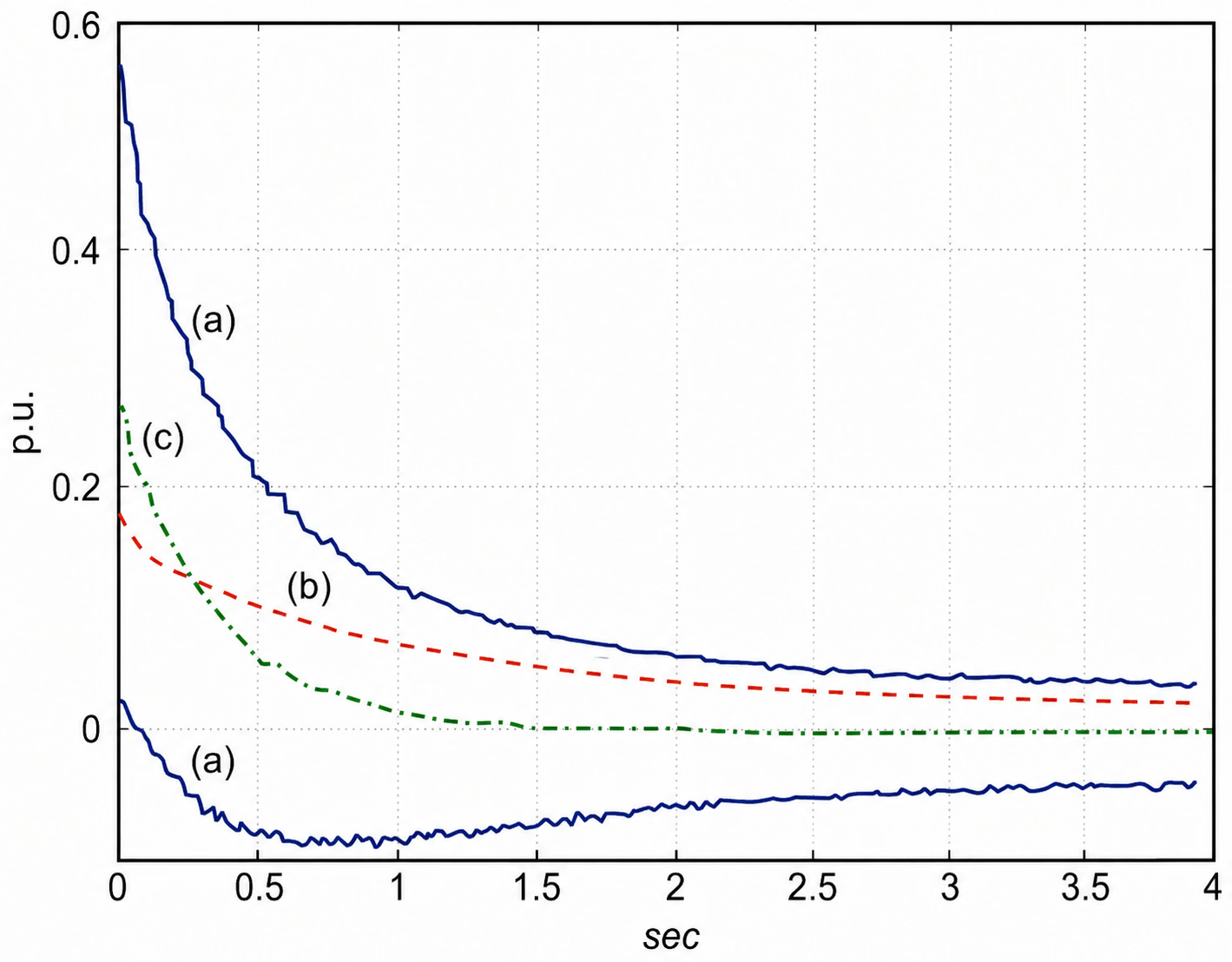
The recorded armature current from a sudden three-phase short-circuit test is not a single simple decaying sinusoid. For parameter determination, it is interpreted as a combination of a decaying symmetrical AC component, a decaying DC-offset component and, depending on the formulation and measurement processing, a second-harmonic component. Separating these components correctly is essential before extracting \(X'_d\), \(X''_d\), \(T'_d\), \(T''_d\) and the armature time constant \(T_a\).

IEEE Std 1110-2019 Figure 15: graphical decomposition of the sudden three-phase short-circuit armature current into its upper and lower envelopes, the decaying symmetrical AC component and the decaying DC-offset component (with the second-harmonic term of the short-circuit-current formulation identified), used to separate the components before fitting the time constants. — **Figure 1 —** Decomposition of the sudden three-phase short-circuit armature current into its components: (a) the upper and lower current envelopes; (b) the symmetrical AC component; (c) the DC-offset component. The separation supports interpretation of the measured waveform before fitting the transient and subtransient time constants.

Use this figure as a fitting and interpretation aid. It should not be treated as a complete conversion method. The sudden three-phase short-circuit test mainly excites the direct-axis response and normally gives stronger information for \(X'_d\), \(X''_d\), \(T'_d\), \(T''_d\) and \(T_a\) than for the q-axis model. Q-axis quantities should only be used where they are supported by suitable tests, manufacturer calculations or frequency-response data.

Section 9

Extracting the reactances and time constants

The phase currents are processed to separate the DC components and obtain the AC rms envelope. The steady-state value is subtracted, leaving the transient-plus-subtransient curve. Plotted on a semi-logarithmic scale, the curve becomes approximately straight once the fast subtransient component has decayed — this later straight line is the transient component. Its zero-time intercept gives \(X'_d\), and its slope gives \(T'_d\) (the time for the transient component to decay to \(1/e \approx 0.368\) of its initial value). Subtracting the transient straight line leaves the early subtransient curve; its intercept gives \(X''_d\) and its slope gives \(T''_d\).

\[ I(t) = I_0\,e^{-t/T} \]

\(I(t)\): the current-envelope component being fitted
\(I_0\): initial (zero-time intercept) value of that component
\(t\): time after the fault instant
\(T\): time constant of the component (\(T'_d\) for the transient part, \(T''_d\) for the subtransient part)

On a semi-logarithmic axis the component is a straight line: its slope gives the time constant \(T\) and its zero-time intercept gives \(I_0\) (and hence the corresponding reactance). The slow component is fitted first; subtracting it isolates the faster one. The fitting interval must be chosen consistently.

The actual current does not follow exactly two ideal exponentials — saturation, eddy currents, noise and construction intervene — so the chosen fitting interval affects the result. Test procedures specify the time range used for fitting so that two engineers analysing the same waveform get the same \(X'_d\) and \(T'_d\). For EMTP® modelling, the extracted values are characteristic parameters derived under a specified procedure, not exact physical constants — one reason equivalent-circuit conversion and validation are still needed.

Confirm the current-trace form before fitting

Before fitting test data, confirm whether the supplied current trace is instantaneous phase current, peak envelope, RMS symmetrical current or per-unit current. Mixing these forms can produce incorrect reactances and time constants — even when the curve fit itself appears visually acceptable.

Section 10

Temperature correction and the armature time constant

Winding resistance changes with temperature, and time constants depend on resistance, so some must be corrected to a reference temperature (copper and aluminium use different constants): higher temperature raises resistance and lowers the time constant. Both stator and field resistance are affected, and an uncorrected value distorts the armature time constant, the field-circuit response and the calculated losses. The d-axis transient short-circuit time constant is commonly corrected; the subtransient time constant often is not, because its physical paths (damper, solid-rotor, eddy-current) do not follow a simple winding-resistance law. The armature time constant is commonly corrected too, often to 75°C, since it depends on armature resistance. The DC offset decays with \(T_a\), determined by extracting the DC components, plotting the equivalent DC magnitude on a semi-log scale and extrapolating to the fault instant (the time to decay to \(1/e\) of the initial value). It should be checked against:

\[ T_a \approx \frac{L_2}{R_a} \]

\(T_a\): armature (DC-offset) time constant
\(L_2\): negative-sequence inductance
\(R_a\): armature resistance

\(T_a\) matters for asymmetrical fault current, the first current peak, breaker making duty, protection performance and the torque offset.

Section 11

Short-circuit variants and q-axis

A second method applies the three-phase short circuit to the armature and simultaneously short-circuits the field — used when the excitation system cannot be represented as a constant low-impedance voltage source during the test (a remote exciter, or one disturbed by heavy transient current). The steady-state armature current then becomes zero because the field is also shorted, and the response is analysed similarly but with the steady excitation term removed; it gives d-axis transient and subtransient information.

As noted above, a no-load sudden short circuit gives mainly d-axis data, so q-axis transient and subtransient quantities need a condition with q-axis flux present. One method runs the machine on load at low voltage with the field shorted and then applies a sudden short circuit; the rotor position must be known (shaft signals) so d- and q-axis components can be separated, and the q-axis current and d-axis voltage at the fault instant give \(X'_q\), \(X''_q\), \(T'_q\), \(T''_q\) where the model supports them. This procedure is more complex and less commonly available.

Section 12

Decrement tests

Open-circuit versus short-circuit time constants

A short-circuit time constant (\(T'_d\), \(T''_d\)) is measured or inferred with the stator shorted, as in the sudden short-circuit test; an open-circuit time constant (\(T'_{d0}\), \(T''_{d0}\)) is measured or inferred with the stator open, as in the voltage-recovery test below. The open-circuit values are the larger of the pair, and the two are not interchangeable. An EMTP® model input field expects one or the other depending on its formulation, so the convention must be checked before entering the data.

Decrement tests derive parameters from the decay or recovery of voltage or current after a switching action, and are especially useful for open-circuit time constants \(T'_{d0}\), \(T''_{d0}\), \(T'_{q0}\), \(T''_{q0}\). In the voltage recovery test, a steady three-phase short circuit is suddenly removed while the machine runs at rated speed with selected excitation; the terminal voltage recovers toward its open-circuit value with transient and subtransient components. The differential voltage (final steady value minus the recovering voltage) is plotted on a semi-log scale: after the first cycles the straight transient line gives \(X'_d\) by its intercept and \(T'_{d0}\) by its slope, and subtracting it leaves the subtransient component for \(X''_d\) and \(T''_{d0}\). If the speed is not exactly rated, the measured voltages must be corrected by the ratio of rated to actual speed, since no-load voltage is proportional to speed — otherwise speed drift is misread as electromagnetic recovery.

Two q-axis decrement procedures give open-circuit q-axis parameters: disconnecting the armature while running asynchronously on load with the field shorted (with rotor-position signals to measure q-axis current and d-axis voltage), or disconnecting at very low slip with a supply of ~5–10% rated voltage and the rotor magnetised along the q-axis. Both need careful rotor alignment — small mechanical errors create large electrical-angle errors, especially in many-pole machines.

Section 13

Standstill frequency response (SSFR)

SSFR is one of the most powerful identification methods. The machine is offline, isolated and at standstill; controlled sinusoidal signals are injected into the stator or field over a range of frequencies, and the resulting voltages and currents give frequency-response functions. Unlike sudden-short-circuit and decrement tests (mostly second-order approximations), SSFR can identify operational inductances and transfer functions over a wide frequency range — the d- and q-axis operational impedances and inductances, the armature-to-field transfer function and transfer impedance, and the field-to-armature effective turns ratio — supporting higher-order equivalent circuits.

SSFR is valuable because it can be done in the factory or on site at low current, avoids the severe mechanical stress of large sudden-short-circuit tests, provides q-axis information more directly, identifies the field response, and gives frequency-domain rather than only time-domain information. For high-quality generator models — shaft torque, subsynchronous resonance (SSR), damping, excitation response — SSFR can be more informative than traditional short-circuit tests alone. The tests are run separately for each axis with the rotor aligned to the d- or q-axis, giving \(Z_d(s)\) and \(Z_q(s)\); the operational inductances follow:

\[ L_d(s) = \frac{Z_d(s) - R_a}{s} \qquad\qquad L_q(s) = \frac{Z_q(s) - R_a}{s} \]

\(L_d(s),\ L_q(s)\): d- and q-axis operational inductances
\(Z_d(s),\ Z_q(s)\): d- and q-axis operational impedances seen from the armature
\(R_a\): DC armature resistance
\(s\): Laplace-domain complex frequency variable
\(s = j\omega\): its sinusoidal (frequency-response) form, with \(\omega\) the angular frequency

The function \(sG(s)\) is often measured rather than \(G(s)\) directly, because it is convenient to measure in the same test.

Section 14

SSFR parameter identification

The d-axis procedure starts from the best estimate of armature leakage inductance (often from the manufacturer), takes the low-frequency limit of \(L_d(s)\) for the synchronous level, and finds the mutual inductance:

\[ L_{ad} = L_d(0) - L_l \qquad\qquad L_{aq} = L_q(0) - L_l \]

\(L_d(0),\ L_q(0)\): low-frequency limits of the operational inductances
\(L_l\): stator leakage inductance
\(L_{ad},\ L_{aq}\): d- and q-axis mutual inductances

The d-axis then uses the armature-to-field transfer impedance for the field-to-armature turns ratio, refers the field resistance to the armature side, chooses the circuit structure, and fits the unknown parameters to reproduce both \(L_d(s)\) and \(sG(s)\). The q-axis is simpler (no field): fit the damper parameters to reproduce \(L_q(s)\). In both cases the mutual inductance is finally adjusted to the unsaturated air-gap-line value using the OCC, because SSFR is run at low current and standstill, where the measured iron-dependent inductance may not match the unsaturated value the model needs. Fitting itself — nonlinear least-squares, pattern search, non-iterative or maximum-likelihood methods — must be judged on physical plausibility (positive resistances, meaningful inductances, realistic time-domain response), not only mathematical error, since noise and different structures can fit the same data differently. The general algorithms that turn these operational inductances into equivalent-circuit parameters are set out on the data-conversion page; here the focus is the SSFR measurement and what it yields.

Section 15

Limitations of SSFR

SSFR is powerful but has limits. It is at standstill, so centrifugal effects on damper windings are absent; at low current, so the magnetic state differs from rated operation, and the inductances are unsaturated — saturation must still come from the OCC. Damper-path contact resistance may differ from running conditions; the DC armature resistance used in the impedance-to-inductance step may not capture higher-frequency eddy losses; the amplifiers must be accurate and linear; rotor alignment can be difficult (especially salient-pole); and noise affects fitting. Salient-pole machines add challenges — a much lower \(L_q/L_d\), a concentrated field winding, a different damper structure, fractional slots per pole, and large electrical-angle errors from small positioning errors — so identification methods developed for round-rotor machines should not be applied without checking their validity. None of this makes SSFR unreliable; it means the results must be interpreted carefully and validated against other data.

Section 16

Online tests

Online tests run while the machine is connected and operating near normal conditions, overcoming some limitations of offline tests because rotation, magnetic state and control interaction are included.

Online frequency response — the excitation is modulated with small sinusoids while running; field voltage/current, terminal voltage, active and reactive power and rotor speed give frequency-response functions, with the machine in its real operating state (but with system interaction, noise and control effects mixed in).
Load rejection — the breaker is opened while running and the terminal voltage, field voltage and field current recorded, under under- and over-excited conditions for different saturation states; it reveals the combined machine, saturation and excitation behaviour, valuable for overvoltage and voltage-response studies (but a significant disturbance, to be planned carefully).
Small-disturbance — minor operating-point changes identify linear parameters around a point without severe stress, useful for normal-operation dynamics across a range of loading.
Large-disturbance — a significant change, often in excitation reference, validates nonlinear models, saturation and excitation response under realistic conditions, but is demanding and needs careful planning.

Online tests are valuable for capturing the operating-condition response and for validating excitation and control interaction, but they do not cleanly isolate individual machine parameters — system conditions, controls and network dynamics are mixed into the measured response. They therefore complement, rather than replace, controlled factory parameter tests.

Section 17

Which test provides which parameter

Table 1 — Typical relationship between synchronous-machine tests and the data they support.
Test	Parameters Provided
Open-circuit characteristic (OCC)	Saturation curve, air-gap line, field-current base, no-load voltage relation
Short-circuit characteristic (SCC)	Steady SC relation; supports X_d and SCR
Slip test	Estimate of X_q
Sudden 3-phase SC at no load	X′_d, X″_d, T′_d, T″_d, T_a
Sudden SC, armature & field shorted	d-axis transient/subtransient where constant excitation can’t be held
Sudden SC on load (low voltage)	X′_q, X″_q, T′_q, T″_q
Voltage recovery	X′_d, X″_d, T′_d0, T″_d0
q-axis decrement	X′_q, X″_q, T′_q0, T″_q0 (where supported)
SSFR	L_d(s), L_q(s), sG(s), field-transfer data, higher-order circuits
Online tests	Operating-condition response, control interaction, validation data

Section 18

Connecting test data to the EMTP® model and validating it

Test results provide characteristic data. The selected EMTP® model structure determines which internal parameters are needed; data conversion then turns the measured characteristics into equivalent-circuit parameters; and validation checks whether the model reproduces the measured response relevant to the study — the sudden short-circuit envelope for a fault study, voltage recovery and saturation for a recovery study, electrical damping and shaft data for torsional work, and field-transfer behaviour for excitation studies. The model should be checked against:

The OCC no-load voltage.
The SCC steady short-circuit current.
The d-axis synchronous reactance \(X_d\) and a reasonable SCR.
The initial short-circuit current (\(X''_d\)).
The transient and subtransient decay (\(T'_d, T''_d\)).
The armature / DC-offset decay (\(T_a\)).
The voltage recovery (\(T'_{d0}, T''_{d0}\)).
The q-axis response where available.
The SSFR response where available.
The field current and field voltage.
Stable no-disturbance operation.

Reproducing these responses matters more than matching every data-sheet number.

Section 19

Common mistakes in test-based parameter determination

Avoid these

Confusing the test procedure with the model parameter — a sudden short-circuit test gives characteristic reactances and time constants, not field leakage inductance directly.
Treating measured characteristic parameters as if they were the final internal equivalent-circuit parameters.
Using open- and short-circuit time constants interchangeably.
Neglecting temperature correction where it is required.
Assuming q-axis parameters are as easy or certain to obtain as d-axis ones.
Fitting the current decay over the wrong time interval.
Mixing RMS, peak and instantaneous quantities.
Using saturated and unsaturated data together without stating the basis.
Relying on an SSFR mathematical fit without time-domain validation.
Accepting an EMTP® model because it runs rather than because it reproduces the measured behaviour.

Section 20

Where this fits in the series

This guide explains where the data used in the data-conversion page comes from. The test procedures provide the OCC/SCC curves, the transient and subtransient time constants, the SSFR functions and the validation traces; the conversion page then turns those test outputs into the internal EMTP® equivalent-circuit parameters. The next page covers the magnetic-saturation model the OCC supports, and the underlying behaviour is detailed in Parameters and Short-Circuit Response over the per-unit equivalent circuits.

Section 21

Suggested report wording

Model statement — for a study report

“The synchronous-machine parameter set was based on the available manufacturer and test data, including steady-state OCC/SCC information, short-circuit and decrement response, voltage-recovery data, SSFR results where available and any relevant online validation records. The test outputs were interpreted as characteristic quantities rather than final internal circuit parameters. Open- and short-circuit time constants, the saturation basis, winding-temperature correction, the RMS/peak convention, q-axis data limitations and model-order suitability were checked before conversion into the EMTP® model. The resulting model was validated against the measured no-load, short-circuit, decay, field and no-disturbance responses relevant to the study.”

Section 22

Main takeaway

Testing is the link between the physical machine and the model

Synchronous-machine parameters are only as reliable as the tests and interpretation behind them. OCC/SCC tests define steady-state and saturation behaviour; sudden short-circuit and decrement tests define transient and subtransient response; SSFR provides frequency-domain information for higher-order models; and online tests support validation. The message: a reliable EMTP® model is not created by entering isolated data-sheet values — the engineer must understand what each test actually measures, how the data converts into equivalent-circuit parameters, and whether the final model reproduces the measured response.

References

The IEEE/IEC test-procedure standards that define these tests, and the standard machine-modelling references.

IEEE Std 115-2009, IEEE Guide for Test Procedures for Synchronous Machines. New York, NY, USA: IEEE.
IEC 60034-4, Rotating Electrical Machines – Part 4: Methods for Determining Synchronous Machine Quantities from Tests. Geneva, Switzerland: International Electrotechnical Commission.
J. A. Martínez-Velasco, Ed., Power System Transients: Parameter Determination, Ch. 5 (Synchronous Machines). Boca Raton, FL, USA: CRC Press, 2010.
IEEE Std 1110-2019 (Revision of IEEE Std 1110-2002), IEEE Guide for Synchronous Generator Modeling Practices and Parameter Verification with Applications in Power System Stability Analyses. Piscataway, NJ, USA: IEEE, 2020.
P. Kundur, Power System Stability and Control. New York, NY, USA: McGraw-Hill, 1994.

Part Seven Reading now

Test Procedures and Parameter Determination

Steady-state, sudden-short-circuit, decrement, SSFR and online tests — and which test yields which reactance, time constant or operational inductance.

Series progress 7 of 9

Part Eight

Magnetic Saturation

The open-circuit characteristic and air-gap line, saturated and unsaturated reactance, and the saturation factor applied to the mutual air-gap inductance.