Data Conversion · EMTP®

Data Conversion Procedures for Synchronous Machine Models

An EMTP®-type synchronous-machine model is built from fundamental circuit parameters — stator leakage inductance, d- and q-axis mutual inductances, field and damper resistances and leakage inductances. Manufacturers rarely give these directly; they give derived quantities (synchronous, transient and subtransient reactances, open- and short-circuit time constants, and sometimes operational inductances from frequency-response tests). Data conversion is the step that moves from the available derived parameters to the internal equivalent-circuit parameters the model needs. The equations may be right and the simulation may converge, but if the conversion is wrong, the simulated machine will not represent the real generator or motor.

Reading time ≈ 35 min · Test data → equivalent-circuit parameters

A reliable EMTP® synchronous-machine model needs three things: a suitable model structure, a consistent set of input parameters, and a defensible conversion procedure from the available data to the fundamental model parameters. This guide is about the third.
Abbreviations used on this page
EMTP®Electromagnetic Transients Program
MVAMegavolt-ampere (apparent-power base)
\(L_d(s),\ L_q(s)\)d- and q-axis operational inductances
\(G(s)\)Armature-to-field transfer function
\(s = j\omega\)Laplace complex frequency (\(\omega\) = angular frequency)
\(L_d, L'_d, L''_d\)d-axis synchronous / transient / subtransient inductance
\(L_q, L'_q, L''_q\)q-axis synchronous / transient / subtransient inductance
\(L_{ad}, L_{aq}\)d- and q-axis mutual (magnetising) inductances
\(L_{al}\)Armature (stator) leakage inductance
\(L_{Fdl}\)Field-damper leakage path (Canay)
\(L_C\)Canay characteristic inductance
\(R_F, R_D\)Field and d-damper resistances
F, D, Q1, Q2Field, d-damper, q-dampers
Key idea
  1. Test reactances and time constants are observed external responses, not internal circuit elements — \(X''_d\) is not an inductor you can drop into the field winding.
  2. A complete second-order d-axis model needs both \(L_d(s)\) and \(G(s)\); without \(G(s)\) the field-damper leakage \(L_{Fdl}\) cannot be uniquely found — unless Canay’s inductance supplies it.
  3. Identify branches by time constant: the larger d-axis time constant is the field winding, the smaller is the damper.
  4. Use the simplest model the data supports, watch the time base (seconds vs per unit), and reject non-physical results such as negative leakage inductance.
Key terms used on this page
01Derived parameter
A test-observed quantity such as \(X'_d\) or \(T''_d\); not a physical circuit element.
02Fundamental parameter
An internal R or L of the equivalent circuit, used directly by the solver.
03Operational data
Frequency-domain functions \(L_d(s)\), \(L_q(s)\), \(G(s)\) from frequency-response tests.
04Classical data
Reactances and time constants from data sheets and stability models.
05Model order
How many rotor circuits are represented on each magnetic axis.
06Armature-to-field \(G(s)\)
How field voltage transfers into d-axis armature flux; identifies the field branch.
07Canay characteristic inductance
\(L_C\): supplies the field-damper leakage when \(G(s)\) is unavailable.
08Field-damper leakage \(L_{Fdl}\)
Flux linking field and damper but not the stator d-axis winding.
09Open- vs short-circuit time constant
Same rotor circuits seen under different stator boundary conditions.
10Field/damper identification
Assigning solved branches by time-constant size (slow = field, fast = damper).

Section 1

Why data conversion is one of the most important steps

The d- and q-axis equivalent circuits describe the complete electrical behaviour of the machine over the intended transient range, and EMTP® solves their voltage and flux-linkage equations directly in the time domain. The problem is that standard machine data is not provided in that form. A test report gives quantities that describe the observed response under particular test conditions — they are not the field leakage inductance, damper leakage inductance, field resistance or damper resistance. Data conversion is the process that reconstructs an equivalent internal circuit from these observed external quantities. The simulation can be perfectly well built and still converge on a machine that does not represent the real one if the conversion behind it is wrong.

Section 2

Derived parameters are not circuit elements

A test report typically lists the d- and q-axis synchronous, transient and subtransient reactances together with the open- and short-circuit time constants:

\[ X_d,\ X'_d,\ X''_d \qquad X_q,\ X'_q,\ X''_q \] \[ T'_d,\ T''_d,\ T'_{d0},\ T''_{d0} \qquad T'_q,\ T''_q,\ T'_{q0},\ T''_{q0} \]

In this notation \(X\) is a reactance and \(T\) a time constant; the subscript \(d\) or \(q\) is the direct or quadrature axis; a prime (\('\)) denotes a transient and a double prime (\(''\)) a subtransient quantity; and a subscript \(0\) denotes an open-circuit value (otherwise it is a short-circuit value). These describe the machine’s observed response, not its internal elements. \(X''_d\), for instance, is not a physical inductor that can be inserted into the field winding — it is the effective d-axis subtransient reactance seen at the stator immediately after a sudden disturbance, produced by the combined effect of the armature leakage, d-axis magnetising inductance, field winding, damper winding and the constraint that rotor flux linkages cannot change instantaneously. Data conversion reconstructs an equivalent internal circuit from these external quantities.

Section 3

Two types of machine data

Available data falls into two broad categories. Operational data — the d-axis operational inductance \(L_d(s)\), the q-axis operational inductance \(L_q(s)\) and the armature-to-field transfer function \(G(s)\) — comes from frequency-response or parameter-identification studies and carries rich information about the internal rotor circuits over frequency. Classical transient and subtransient data — reactances and open-/short-circuit time constants — is what most data sheets and stability models provide; it is less complete but often enough for simplified equivalent circuits. The conversion procedure depends on which set is available: a complete conversion is only possible when the data contains enough information to identify the selected model structure.

In practice the available data falls on a spectrum, and the conversion method follows it:

  • Best case — operational inductances \(L_d(s)\), \(L_q(s)\) and the transfer function \(G(s)\): the complete model can be identified.
  • Intermediate case — operational inductances plus Canay’s characteristic inductance \(L_C\): the complete d-axis model can still be recovered without \(G(s)\).
  • Common case — classical reactances and time constants only: usually enough for a simplified model.
  • Weak case — incomplete manufacturer data needing assumptions: convert with caution and document every assumption.

Section 4

Fundamental parameters required by the circuits

The conversion must deliver the internal building blocks of the equivalent circuits:

\[ \text{d-axis:}\quad L_{al},\ L_{ad},\ L_{Fl},\ L_{Dl},\ L_{Fdl},\ R_F,\ R_D \] \[ \text{q-axis:}\quad L_{aq},\ L_{Q1l},\ L_{Q2l},\ R_{Q1},\ R_{Q2} \]
\(L_{al}\)
stator leakage inductance
\(L_{ad},\ L_{aq}\)
d- and q-axis armature mutual inductances
\(L_{Fl},\ L_{Dl}\)
field and d-damper leakage inductances
\(L_{Fdl}\)
field-damper leakage path (links field and damper, not the stator d-axis)
\(R_F,\ R_D\)
field and d-damper resistances
\(L_{Q1l}, L_{Q2l},\ R_{Q1}, R_{Q2}\)
q-axis damper leakage inductances and resistances

These are not always visible to the user, but they determine the transient response.

The conversion is a parameter-identification problem

The engineer chooses a circuit structure, then calculates the branch parameters so that the equivalent circuit reproduces the supplied reactances, time constants or frequency-response functions. If the chosen structure cannot reproduce the data using positive passive elements, the conversion produces warning signs such as negative leakage inductance or unrealistic resistance — a signal to revisit the data or the model, not to accept the numbers.

Section 5

Model order and what it means

“Model order” is how many rotor circuits are represented on each magnetic axis. A simple d-axis model has only the field circuit — it can reproduce the main transient behaviour but not detailed subtransient behaviour. A second-order d-axis model adds one d-axis damper, allowing both transient and subtransient effects. A more detailed model adds a second d-axis damper for greater flexibility in fitting frequency response. On the q-axis there is no field winding; the response is carried by dampers, with a second-order q-axis model normally using two q-axis circuits (simpler machines may use one, more complex ones more). The correct order depends on the study and the data — a high-order model cannot be justified without enough test data to determine its parameters.

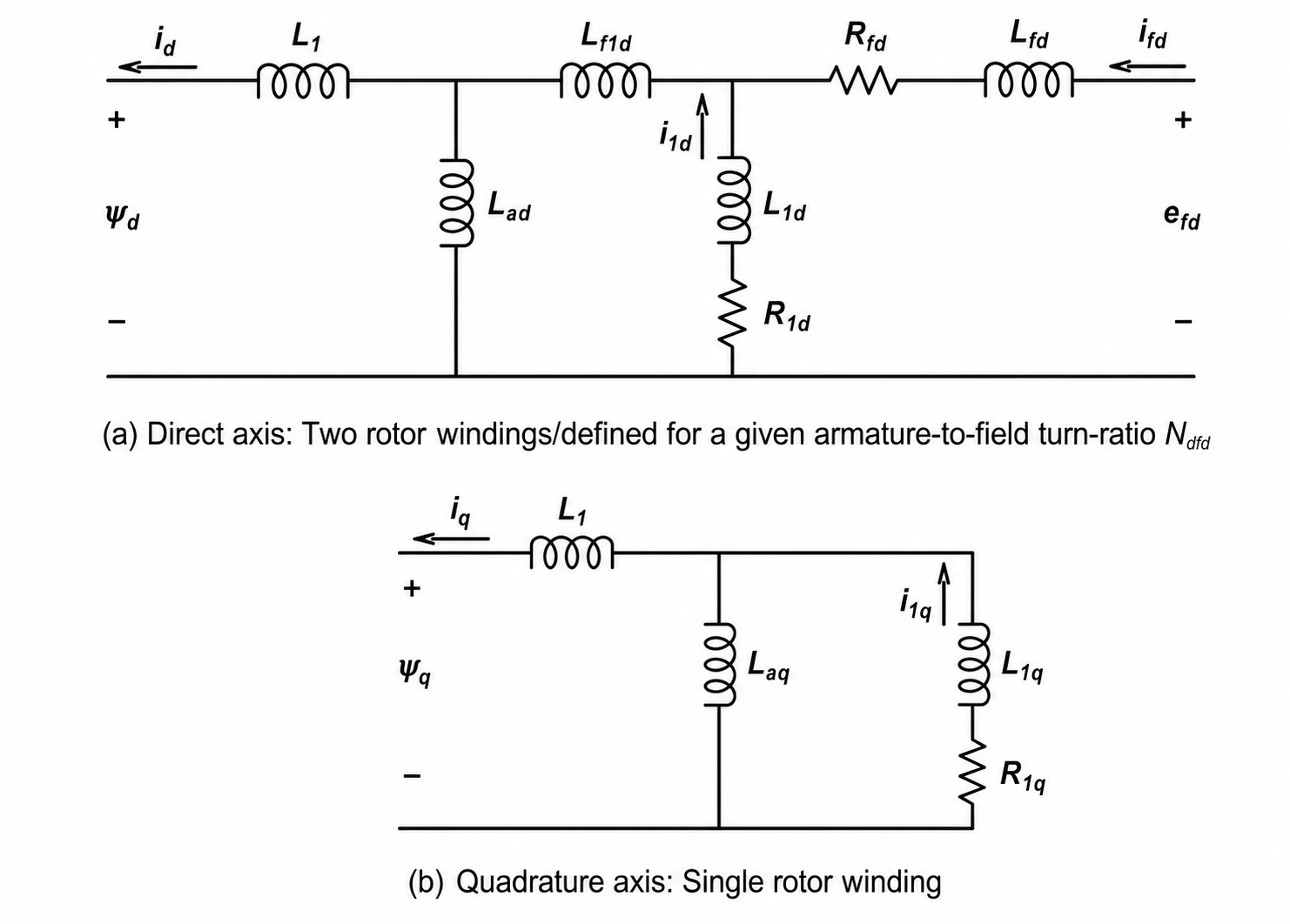
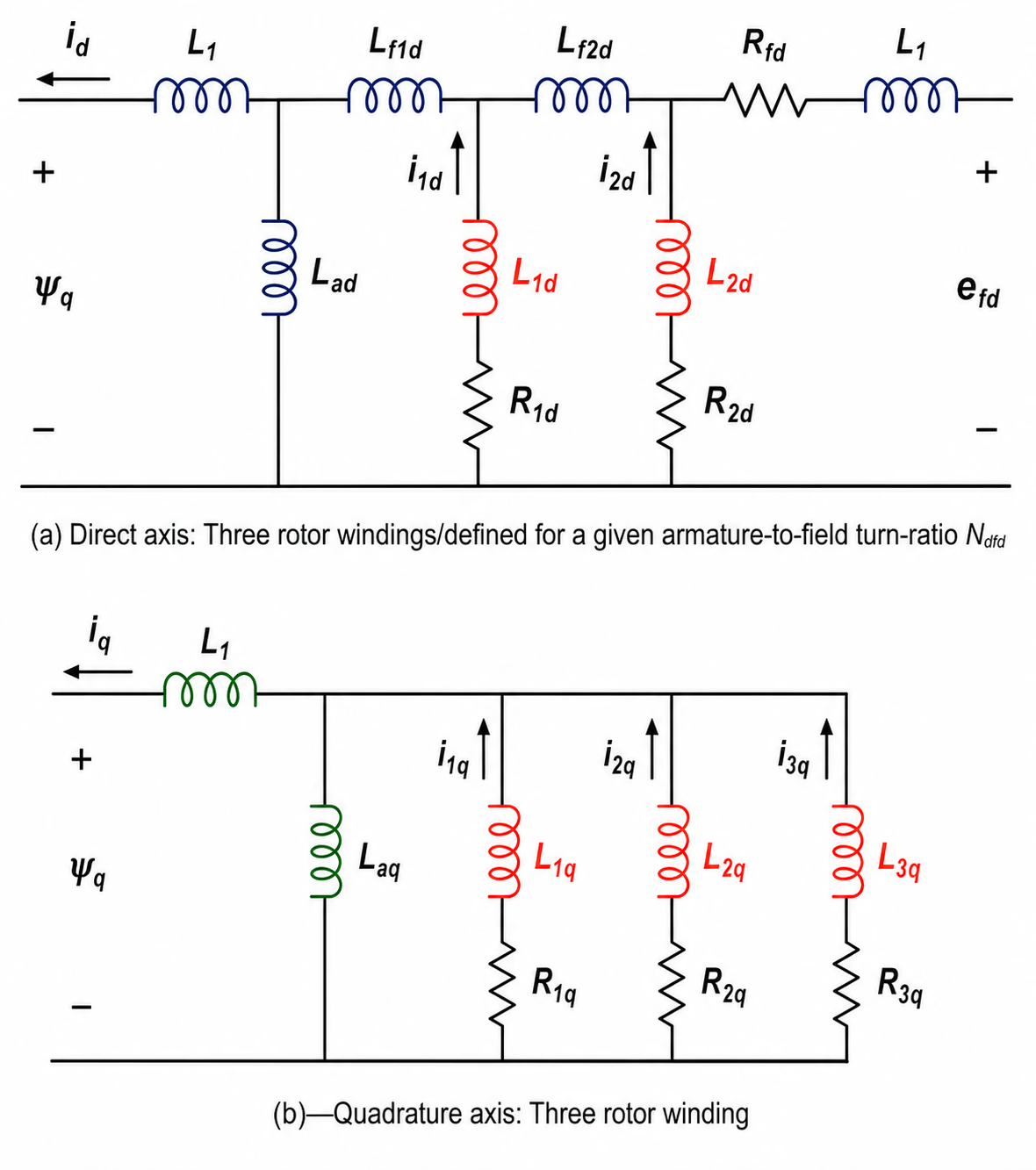
In the Model N.M notation, N represents the number of equivalent rotor windings on the direct axis and M represents the number of equivalent rotor windings on the quadrature axis. For example, Model 2.1 represents the d-axis using the field winding plus one d-axis damper winding, and the q-axis using one q-axis damper winding. Model 3.3 uses a higher-order representation with additional damper branches. Higher order is not automatically better; it is useful only when the available data can identify the additional parameters.

Before any conversion is performed, the model structure must be selected. The same set of terminal measurements does not uniquely define every internal field, damper and leakage parameter. The engineer must therefore choose a d-axis and q-axis equivalent-circuit order that is supported by the available data. Lower-order models are suitable when only classical reactances and time constants are available; higher-order models require stronger test support, such as frequency-response data or manufacturer-derived rotor information.

IEEE Std 1110-2019 Figure 12: Model 2.1 d- and q-axis equivalent circuits referred to the stator terminals - the d-axis with the field winding and one d-axis damper branch, the q-axis with one q-axis damper branch.
Figure 1 — Model 2.1 equivalent-circuit structure referred to the stator terminals. This lower-order structure represents the d-axis with the field winding and one d-axis damper path, and the q-axis with one q-axis damper path. It is a common practical model when the available data supports transient and subtransient behaviour but not a fully higher-order fit.
IEEE Std 1110-2019 Figure 13: Model 3.3 d- and q-axis equivalent circuits referred to the stator terminals - a higher-order structure with additional d-axis and q-axis damper branches.
Figure 2 — Model 3.3 equivalent-circuit structure referred to the stator terminals. This higher-order structure contains additional d-axis and q-axis damper branches, allowing a more detailed fit to operational inductance or frequency-response data where such data is available and reliable.

Use these figures to clarify the difference between model structure and parameter value. A parameter such as armature leakage inductance, field leakage, damper leakage or armature-to-field turns ratio is not always uniquely recoverable from terminal tests alone. The selected model can still reproduce terminal behaviour if the remaining parameters are calculated consistently, but the internal field current, damper current and torque behaviour may depend on the chosen structure. Therefore, model order, leakage assumption, field-current base and q-axis representation must be stated before the conversion result is accepted.

Section 6

Complete second-order d-axis model from G(s) and Ld(s)

The most complete second-order d-axis conversion is possible when both \(L_d(s)\) and \(G(s)\) are available, together with the stator leakage inductance \(L_{al}\). This is a strong data set: \(L_d(s)\) describes how d-axis armature flux responds to d-axis stator current over frequency, while \(G(s)\) describes how field voltage affects d-axis armature flux — together covering both the armature and field sides. The first step is the mutual inductance:

\[ L_{ad} = L_d - L_{al} \] \[ DS = (T''_{d0} + T'_{d0}) - (T''_d + T'_d) \qquad DP = (T''_{d0}\,T'_{d0}) - (T''_d\,T'_d) \]
\(L_{ad}\)
d-axis mutual inductance (\(L_d\) synchronous, \(L_{al}\) leakage)
\(DS,\ DP\)
intermediate sum- and product-difference quantities
\(T''_{d0}, T'_{d0}\)
open-circuit subtransient and transient time constants
\(T''_d, T'_d\)
short-circuit subtransient and transient time constants

Open- and short-circuit time constants observe the same rotor circuits under different stator boundary conditions, so their differences contain information about the stator–rotor coupling. When \(G(s)\) is available, an additional time constant on the armature-to-field path can be identified, letting the complete second-order circuit be solved — including the field-damper leakage \(L_{Fdl}\) — for the full set \(R_F, R_D, L_{Fl}, L_{Dl}, L_{Fdl}, L_{ad}\). This is the preferred method when high-quality operational data exists.

In summary, the complete d-axis conversion proceeds in clear steps:

  1. Select the model order (here a second-order d-axis: the field plus one damper).
  2. Fix the stator leakage inductance \(L_{al}\) from the manufacturer or a reasoned estimate.
  3. Read the synchronous, transient and subtransient limits from \(L_d(s)\).
  4. Form the d-axis mutual inductance \(L_{ad}=L_d-L_{al}\).
  5. Use \(G(s)\) to identify the field branch and the field-damper coupling, then solve for the field and damper branch parameters.
  6. Check the time constants and confirm every branch resistance and leakage inductance is positive and physically meaningful.
  7. Validate by reconstructing \(L_d(s)\) and \(G(s)\) from the solved circuit and comparing with the measured data.

Section 7

Why G(s) matters

\(G(s)\) gives information \(L_d(s)\) alone cannot. The operational inductance describes how d-axis stator current relates to d-axis armature flux for a specified field-voltage condition, but it does not fully identify how the field voltage transfers into the armature flux. \(G(s)\) relates field voltage directly to d-axis armature flux, letting the field branch and the field-damper coupling be identified more completely. Without \(G(s)\), some internal distinctions cannot be determined uniquely, and a simplified model or an additional quantity such as Canay’s characteristic inductance is needed.

In one line

\(L_d(s)\) tells us how the armature sees the machine; \(G(s)\) helps tell us how the field circuit communicates with the armature.

Section 8

Simplified second-order d-axis model (no G(s))

In many projects \(G(s)\) is not available — only \(L_d(s)\), or the standard reactances and time constants. The complete model then cannot be uniquely identified without an extra quantity, so the usual simplification omits the field-damper leakage path \(L_{Fdl}\): the field, d-damper and stator d-axis windings are assumed to link a single ideal mutual air-gap flux \(L_{ad}\). This is widely used in stability software and many transient studies — often adequate, though not physically identical to the complete model.

\[ \text{simplified:}\quad L_{FD} = L_{ad} \qquad\qquad \text{with Canay:}\quad L_{FD} = L_{ad} + L_{Fdl} \]
\(L_{FD}\)
effective mutual coupling between the field and d-axis damper path
\(L_{ad}\)
d-axis mutual air-gap inductance
\(L_{Fdl}\)
field-damper leakage path (zero in the simplified model)

The simplified assumption removes one internal degree of freedom and lets the remaining field and damper parameters be found from \(L_d(s)\) or the time-constant data — producing \(R_F, R_D, L_{Fl}, L_{Dl}, L_{ad}\) but not an independently identified \(L_{Fdl}\).

The simplified conversion uses the same idea as the complete method with fewer unknowns: form \(L_{ad}=L_d-L_{al}\), then use \(DS\) and \(DP\) to build a second-order equation whose two roots are the rotor-circuit time constants. The roots do not say which branch is which, so the identification rule is by magnitude: the branch with the larger effective time constant is the field winding (slower transient), the branch with the smaller time constant is the damper (rapid subtransient). Swapping them can reproduce some algebraic quantities but give a physically wrong response. The simplified model is not automatically wrong, but it is less constrained than the complete conversion: it loses the independent field-damper leakage path, so it should not be trusted where that coupling materially affects the result — detailed field/damper interaction, shaft-torque, damping or subsynchronous studies, or solid-rotor machines — where the complete or Canay-corrected model is preferred.

Section 9

Canay’s characteristic inductance

Canay’s characteristic inductance \(L_C\) recovers a more complete d-axis model when \(G(s)\) is unavailable. The difficulty without \(G(s)\) is that the field-damper leakage path cannot be uniquely identified; \(L_C\) supplies the missing information. In the d-axis circuit, \(L_{Fdl}\) represents flux linking both the field and the damper but not the stator d-axis winding — important where short-pitched damper circuits or solid-rotor iron paths make the single-mutual-flux assumption inaccurate. When \(L_C\) is available, the complete second-order d-axis model can be derived from \(L_d(s)\), \(L_{al}\) and \(L_C\) even without \(G(s)\): form \(L_{ad}=L_d-L_{al}\), determine \(L_{Fdl}\) from the relationship between \(L_C\), \(L_{al}\), \(L_{ad}\) and \(L_{Fdl}\), use the corrected coupling \(L_{FD}=L_{ad}+L_{Fdl}\), then solve the two rotor branches and identify them by time constant as before. This is more physically complete than the simplified model, but it needs reliable \(L_C\) data — useful only when its value is consistent with the same base, saturation condition and time-constant convention as the rest of the data set. Canay’s inductance does not by itself rescue a conversion built on inconsistent data.

The practical meaning

Canay’s characteristic inductance restores part of the internal coupling information that is lost when the field-voltage transfer function is unavailable.

Section 10

Caution: negative calculated parameters

In some conversions — especially with incomplete data or a model structure that does not match the machine — calculated leakage inductances can come out negative. A negative value does not automatically mean the algebra is wrong; it may mean the chosen circuit is trying to fit a response it cannot represent with positive passive elements. Likely causes include inconsistent manufacturer data, mixed saturated/unsaturated parameters, a wrong base conversion, the wrong time-constant type (open- vs short-circuit), too simple a model structure, an inappropriate leakage assumption, or data fitted over an incompatible frequency range. A negative leakage inductance should never be accepted blindly — it should trigger a review of the data set, the model, the bases and the conversion assumptions.

Section 11

Second-order q-axis conversion

The q-axis conversion mirrors the simplified d-axis conversion, but with no field winding — only the stator q-axis winding and the q-axis dampers (representing rotor current paths and solid-rotor effects). Start from the mutual inductance:

\[ L_{aq} = L_q - L_{al} \]
\(L_{aq}\)
q-axis mutual inductance
\(L_q\)
q-axis synchronous inductance
\(L_{al}\)
armature leakage inductance

The q-axis operational inductance \(L_q(s)\), or the equivalent q-axis transient/subtransient data, then yields \(R_{Q1}, R_{Q2}, L_{Q1l}, L_{Q2l}\). Because there is no field, there is no field/damper identification step — the two branches are simply dampers with different decay rates. For a simpler q-axis structure (a laminated salient-pole machine with one q-axis damper) the second branch may be meaningless, and the model should be simplified rather than forcing a two-branch q-axis without supporting data.

Section 12

Using classical transient/subtransient data

When operational functions are unavailable, the conversion uses transient and subtransient inductances and time constants. The key is that open- and short-circuit time constants are not independent — they are linked through the transient and subtransient inductances — so a missing set can often be computed from the other, provided the inductances are known. For the simplified second-order d-axis model, three data sets are equivalent if the required inductances are known:

  • Set A — \(T'_d, T''_d, T'_{d0}, T''_{d0}\): both open- and short-circuit time constants directly.
  • Set B — \(L'_d, L''_d, T'_{d0}, T''_{d0}\): transient/subtransient inductances + open-circuit time constants; the short-circuit set is derived.
  • Set C — \(L'_d, L''_d, T'_d, T''_d\): inductances + short-circuit time constants; the open-circuit set is derived.

This is useful because manufacturers provide different combinations — the conversion reconstructs the missing time-constant set, provided the model’s assumptions hold. The same idea applies to the q-axis where the model supports q-axis transient and subtransient behaviour; but the engineer must confirm the q-axis model is appropriate, and not invent a second q-axis dynamic branch (a separate \(T'_q\) or \(L'_q\)) without supporting evidence.

Section 13

Time constants in seconds and per unit

A common source of error is the treatment of time. Test reports give time constants in seconds, but some conversion algorithms use per-unit time, and the conversion depends on the base angular frequency:

\[ \omega_B = 2\pi f_B \qquad t_B = \frac{1}{\omega_B} \qquad T_{\text{pu}} = \omega_B\,T_{\text{s}} \]
\(\omega_B\)
base electrical angular frequency (rad/s)
\(f_B\)
base frequency (Hz)
\(t_B\)
base time (\(=1/\omega_B\))
\(T_{\text{s}}\)
time constant in seconds
\(T_{\text{pu}}\)
the same time constant in per-unit time

A time constant in seconds converts to per-unit time by multiplying by \(\omega_B\) (equivalently dividing by \(t_B\)); the inverse applies the other way. This must be handled consistently — a time-base error changes rotor resistances and damping dramatically. For a 50 Hz machine \(\omega_B = 2\pi\times 50\); for 60 Hz, \(\omega_B = 2\pi\times 60\). EMTP® input fields may expect seconds even when the internal equations are normalised, so confirm which form the program wants and state the convention used.

Section 14

Practical conversion workflow

  1. Identify the available data type (operational functions, classical reactances/time constants, open- or short-circuit values, Canay’s inductance, or only partial data).
  2. Select the model structure (simplified or complete d-axis; one- or two-damper q-axis; higher order).
  3. Confirm all bases — rated MVA, voltage and frequency, the stator leakage inductance, the saturated/unsaturated status, and the reactance-vs-inductance form.
  4. Confirm whether the time constants are open-circuit or short-circuit, and whether time is in seconds or per unit.
  5. Calculate the d-axis and q-axis mutual inductances \(L_{ad}=L_d-L_{al}\) and \(L_{aq}=L_q-L_{al}\).
  6. Derive or reconstruct the required time constants where the model assumptions allow.
  7. Solve for the rotor-branch time constants.
  8. Convert branch time constants into rotor resistances and leakage inductances.
  9. Assign branches to field and damper by physical interpretation (larger d-axis time constant → field; smaller → damper).
  10. Check the derived parameters — positive resistances, meaningful inductances, expected reactance order.
  11. Test the model in EMTP®: a no-disturbance case, then a short circuit, confirming the current envelope follows the expected subtransient, transient and steady-state behaviour.

Section 15

What the conversion should reproduce

A correctly converted model should reproduce the machine’s characteristic behaviour. For a sudden three-phase short circuit: the initial symmetrical current consistent with the subtransient reactance; the early decay with the subtransient time constant; the slower decay with the transient time constant; the final value with the synchronous reactance; and the DC-offset decay with the armature time constant. The field-current response should be physically reasonable, the damper-current response should decay rapidly, and the electromagnetic torque should be plausible and free of numerical artefacts caused by poor conversion. If these are not reproduced, review the conversion before drawing project conclusions.

Note that different parameter sets can reproduce a similar terminal short-circuit current while giving different internal field current, damper current or torque behaviour. So when the study needs internal torque, damping or excitation behaviour, the conversion must be judged on those internal responses, not on terminal current alone. As a quick sanity check the reactances should also order correctly, \(X''_d \le X'_d \le X_d\) (and similarly on the q-axis).

Section 16

Choosing between simplified and complete models

The simplified model suits cases where the data cannot support more detail and the study does not need accurate internal field-damper coupling. The complete model is preferable when operational data or Canay’s inductance is available; when detailed field/damper interaction matters; for severe generator transients; for shaft-torque, damping or subsynchronous-interaction studies; or for solid-rotor generators with significant rotor-current paths. Use the simplified model with caution when the missing leakage path could materially affect the result — but do not use the complete model simply because it is more sophisticated: if the input data is unreliable, the extra detail only adds a false sense of accuracy.

Section 17

Data quality and engineering responsibility

Conversion is not a purely automatic exercise — it needs judgement. Two data sets may both look complete, yet one is saturated and the other unsaturated; one on the machine base, the other on a system base; one with open-circuit time constants, the other short-circuit; one assuming a different q-axis model; one from a factory test, the other from a generic database. Before converting, ask: What is the source? Which standard or test method? Saturated or unsaturated? All on the same base? Open- or short-circuit time constants? Does the q-axis data support the model? Is Canay’s inductance available? Are frequency-response data available? Are any values estimated? Are the resulting parameters physically realistic? The conversion should be documented — especially for generator-duty, protection, transient-stability, subsynchronous-resonance or equipment-specification studies. On saturation specifically: saturated and unsaturated reactances must not be mixed, \(X_d\) may be quoted on either basis, and the conversion must state which — the saturation curves themselves belong to the magnetic-saturation page.

Terminal measurements alone may reproduce terminal current and voltage behaviour while leaving some internal parameter allocations non-unique. This is especially important for leakage inductance, field-current referral and damper-branch allocation. The final conversion should therefore be checked not only against terminal short-circuit current, but also against field-current response, q-axis behaviour where available, torque response, damping behaviour and no-disturbance stability.

Section 18

Common modelling mistakes

Avoid these
  • Treating manufacturer reactances as if they were the final branch inductances.
  • Converting data without confirming the base MVA and voltage.
  • Mixing saturated and unsaturated quantities.
  • Mixing open-circuit and short-circuit time constants.
  • Mixing time constants given in seconds with those in per-unit time.
  • Using a complete second-order model when the data only supports a simplified one.
  • Ignoring a negative leakage inductance or an unrealistic resistance instead of reviewing the data and model.
  • Using Canay’s characteristic inductance without checking its data basis.
  • Inventing q-axis transient data only to fill a model input field.
  • Accepting a black-box software conversion without validating the response.

Section 19

EMTP® implementation perspective

In an EMTP®-type program the user may not see every conversion step — the software may ask for reactances and time constants and internally compute the equivalent-circuit parameters. Even then, the engineer remains responsible for data quality and the modelling choice, and should know which model structure the software uses, whether it is simplified or complete, whether Canay’s inductance is included, whether time constants are open- or short-circuit, whether values are in seconds or per unit, whether reactances are saturated or unsaturated, and whether the q-axis model matches the available data. A black-box conversion should not be accepted without validation.

Section 20

Where this fits in the series

This guide is the conversion step of the synchronous-machine series. The previous page, Parameters and Short-Circuit Response, explains the characteristic reactances and time constants; this page converts those into the d-axis and q-axis equivalent-circuit parameters built on the per-unit equivalent circuits. The following pages explain how the data is obtained, in Test Procedures for Parameter Determination, and how magnetic saturation is represented.

Section 21

Suggested report wording

Model statement — for a study report

“The synchronous-machine manufacturer/test data was converted into the equivalent-circuit parameters required by the EMTP® model using the selected d-axis and q-axis model structure. The conversion considered the available operational or classical data, the stator leakage assumption, the saturated/unsaturated basis, the open- or short-circuit time-constant convention, the seconds-to-per-unit time base and any available Canay characteristic inductance. The resulting field and damper branch parameters were checked for positive resistance, physically meaningful leakage inductance, correct reactance ordering, plausible time constants, agreement with the expected short-circuit current envelope and stable no-disturbance operation.”

Section 22

Main takeaway

A model is only as reliable as the data conversion behind it

Data conversion is the bridge between measured or manufacturer characteristic data and the internal EMTP® equivalent circuit. It is not a mechanical spreadsheet exercise — it is a modelling decision that controls the simulated fault current, torque, damping and voltage response. A reliable conversion requires the correct model order, consistent bases, the correct time-constant convention, a clear saturation basis, physically meaningful branch values and validation against the expected machine response. The message: a numerically accepted parameter set is not enough — it must also make physical sense, and the conversion method must match the available data, the model structure and the transient phenomenon being studied.

References

References

The reference text for the conversion procedures, Canay’s parameter-determination work, and the standard machine-modelling references.

  1. J. A. Martínez-Velasco, Ed., Power System Transients: Parameter Determination, Ch. 5 (Synchronous Machines). Boca Raton, FL, USA: CRC Press, 2010.
  2. I. M. Canay, “Determination of the model parameters of machines from the reactance operators \(x_d(p)\), \(x_q(p)\),” IEEE Transactions on Energy Conversion, vol. 8, no. 2, Jun. 1993.
  3. IEEE Std 1110-2019 (Revision of IEEE Std 1110-2002), IEEE Guide for Synchronous Generator Modeling Practices and Parameter Verification with Applications in Power System Stability Analyses. Piscataway, NJ, USA: IEEE, 2020.
  4. IEEE Std 115-2009, IEEE Guide for Test Procedures for Synchronous Machines. New York, NY, USA: IEEE.
  5. P. Kundur, Power System Stability and Control. New York, NY, USA: McGraw-Hill, 1994.

Nine-Part Technical Series

Synchronous Machine Modelling in EMTP®

A nine-part guide to representing the synchronous machine in EMTP® — from the modelling overview and EMT representation, through the dq0 transformation, per-unit equivalent circuits, parameters, data conversion and tests, to magnetic saturation and high-frequency/shaft modelling.

Part Six Reading now

Data Conversion Procedures

Converting manufacturer and test data into the fundamental equivalent-circuit parameters — operational inductances, model order, Canay’s characteristic inductance and validation.

Series progress 6 of 9