Parameters & Short-Circuit Response

Synchronous Machine Parameters and Short-Circuit Response

The per-unit machine equations need fundamental electrical parameters — the resistances and inductances of the stator, field and damper circuits inside the d- and q-axis models. Those are rarely measured directly. A manufacturer supplies characteristic data — synchronous, transient and subtransient reactances, open- and short-circuit time constants, armature resistance and saturation data — which must be converted into the internal equivalent-circuit parameters an EMTP®-type program uses. The clearest way to understand that data is to watch what happens when a sudden three-phase short circuit is applied to the terminals of an unloaded machine: the response moves from subtransient, through transient, to steady state, and in doing so defines the parameters themselves.

Reading time ≈ 36 min · Reactances, time constants & the short-circuit response

The machine may look simple in the network diagram, but its internal response during a transient is controlled by the field circuit, the damper circuits, the magnetic flux linkages and the winding resistances. If those internal parameters are wrong, the simulated fault current, torque, voltage recovery and damping can all mislead. Parameter conversion — turning test/manufacturer characteristic data into equivalent-circuit values — is therefore a critical part of synchronous-machine modelling, and the three-phase short circuit is the event that makes the parameters intelligible.

Abbreviations used on this page

EMTP®Electromagnetic Transients Program

EMTElectromagnetic transient

MVAMegavolt-ampere (apparent-power base)

\(X_d, X'_d, X''_d\)d-axis synchronous, transient, subtransient reactance

\(X_q, X'_q, X''_q\)q-axis synchronous, transient, subtransient reactance

\(L_d, L'_d, L''_d\)corresponding d-axis inductances (\(X=\omega L\))

\(L_q, L'_q, L''_q\)corresponding q-axis inductances

\(T'_d, T''_d\)d-axis short-circuit transient / subtransient time constants

\(T'_{d0}, T''_{d0}\)d-axis open-circuit time constants

\(T_a\)Armature (DC-offset) time constant

\(L_2\)Negative-sequence inductance

\(L_d(s)\)d-axis operational (frequency-dependent) inductance

AC / DCFundamental-frequency and offset current components

RMSRoot mean square

Key idea

The reactances and time constants describe the short-circuit response, not internal components — they are read from the machine’s subtransient, transient and steady-state behaviour, not measured directly.
A sudden three-phase short circuit decays in three stages: subtransient (dampers), transient (field), steady state (synchronous) — giving \(X''<X'<X\).
The reactances are effective values for different time scales; the operational inductance \(L_d(s)\) shows the same machine looking different to a slow vs a fast disturbance.
Use the simplest model the data supports: subtransient parameters for close-up faults; transient/synchronous for stability; don’t add rotor branches you cannot justify.

Key terms used on this page

01Subtransient reactance

\(X''_d\): the effective reactance in the first cycles, set by the damper circuits.

02Transient reactance

\(X'_d\): the effective reactance after dampers decay, governed by the field circuit.

03Synchronous reactance

\(X_d\): the steady-state reactance after all rotor transients have decayed.

04DC offset

The unidirectional component preserving the initial phase flux at the fault instant.

05Short-circuit time constant

Decay rate of a rotor-current mode with the stator short-circuited.

06Open-circuit time constant

Decay rate with the stator open; usually larger than the short-circuit value.

07Armature time constant

\(T_a=L_2/R_a\): sets the decay of the DC offset.

08Operational inductance

\(L_d(s)\): the effective inductance as a function of frequency.

09Negative-sequence inductance

\(L_2\approx(L''_d+L''_q)/2\): seen by the DC-offset / negative-sequence component.

10Parameter conversion

Deriving equivalent-circuit R and L from test reactances and time constants.

Section 1

What the characteristic parameters are

Manufacturer and test data for a synchronous machine usually does not give the internal stator, field and damper branch parameters directly. Instead, it gives characteristic quantities: synchronous, transient and subtransient reactances, open- and short-circuit time constants, armature resistance and saturation data. The sudden three-phase terminal short circuit is the clearest way to understand these quantities, because the current naturally passes through subtransient, transient and steady-state periods — and in doing so it defines the parameters themselves. Converting the characteristic data into the internal equivalent-circuit parameters is a separate step, set out on the next data-conversion page; this page is about what the parameters mean and how the short-circuit response reveals them.

Section 2

Why the three-phase short circuit is important

A sudden three-phase short circuit at the terminals of an unloaded machine is one of the most informative events in machine modelling: it shows the machine moving from subtransient, through transient, to steady-state short-circuit behaviour. Before the fault the stator is open and the field current produces a rotating flux that each phase winding links sinusoidally as the rotor turns. At the instant of the short circuit the terminal voltage is forced to nearly zero, but the winding flux linkages cannot change instantaneously — so the stator currents take whatever form is needed to preserve the initial flux linkages. That is the physical reason the short-circuit current does not jump straight to its steady-state value: the machine first behaves according to its stored magnetic energy and rotor-circuit constraints, and only as the induced field and damper currents decay does the current approach steady state. The short-circuit response therefore contains exactly the information needed to define the transient and subtransient parameters.

Section 3

Components of the short-circuit current

Each stator phase current after the fault generally contains two parts. The fundamental-frequency AC component is the balanced short-circuit current associated with the rotating field and the machine internal impedance; its amplitude is not constant — it starts high, decays rapidly in the subtransient period, more slowly in the transient period, and finally settles at the steady-state value. The DC offset component appears because the fault can occur at any point on the voltage wave: the initial flux linkage in each phase depends on the switching instant, and the DC offset is what preserves that initial flux immediately after the fault.

For a balanced three-phase fault the AC components are balanced; the per-phase DC offsets differ but sum to zero at every instant, because the three-phase winding system stays balanced as a whole. The rotor responds too: the stator short-circuit currents try to change the rotor flux linkages, and the field and damper windings carry induced currents to oppose those changes — which is why the rotor circuits are essential for accurate short-circuit modelling.

\[ I_{AC}(t) = I_{ss} + (I' - I_{ss})\,e^{-t/T'_d} + (I'' - I')\,e^{-t/T''_d} \] \[ i_{dc}(t) = I_{dc}\,e^{-t/T_a} \qquad I'' \approx \frac{E}{X''_d},\;\; I' \approx \frac{E}{X'_d},\;\; I_{ss} \approx \frac{E}{X_d} \]

\(I_{AC}(t)\): RMS symmetrical AC current envelope at time \(t\)
\(I'',\ I',\ I_{ss}\): initial subtransient, transient and steady-state AC current levels
\(E\): constant internal voltage (the pre-fault terminal voltage of the unloaded machine)
\(T''_d,\ T'_d\): d-axis subtransient and transient short-circuit time constants
\(i_{dc}(t),\ I_{dc}\): DC offset and its initial value (set by the fault inception angle, up to \(\sqrt{2}\,I''\))
\(T_a\): armature time constant (DC-offset decay)

\(I_{AC}\) is the RMS symmetrical envelope; the actual instantaneous phase current is this AC component plus the decaying DC offset \(i_{dc}\). The first peak is therefore higher than the symmetrical value — with full offset it can approach twice it — so first-peak (breaker making) duty must not be read from the symmetrical RMS curve alone. Always state whether a quoted current is RMS symmetrical, peak instantaneous, per-unit, phase or line.

Section 4

Subtransient, transient and steady-state periods

The AC component divides into three regions. The subtransient period (first few cycles) has a high, rapidly decaying current — the damper circuits give low-impedance paths, so the apparent reactance is initially low. The transient period follows: after the fastest damper effects decay, the current decays more slowly under the field winding and slower rotor circuits, and the apparent reactance has risen to the transient value. The steady-state period reaches a constant current set by the synchronous reactance and excitation. The three levels satisfy:

\[ X''_d < X'_d < X_d \qquad L''_d < L'_d < L_d \qquad X = \omega L \]

\(X''_d,\ L''_d\): subtransient reactance / inductance (first cycles)
\(X'_d,\ L'_d\): transient reactance / inductance (following cycles)
\(X_d,\ L_d\): synchronous reactance / inductance (steady state)
\(\omega\): electrical angular frequency; reactance and inductance are related by \(X=\omega L\)

The lower the effective inductance, the higher the current — so the first cycles are governed by the subtransient inductance, the next by the transient inductance, and the final value by the synchronous inductance.

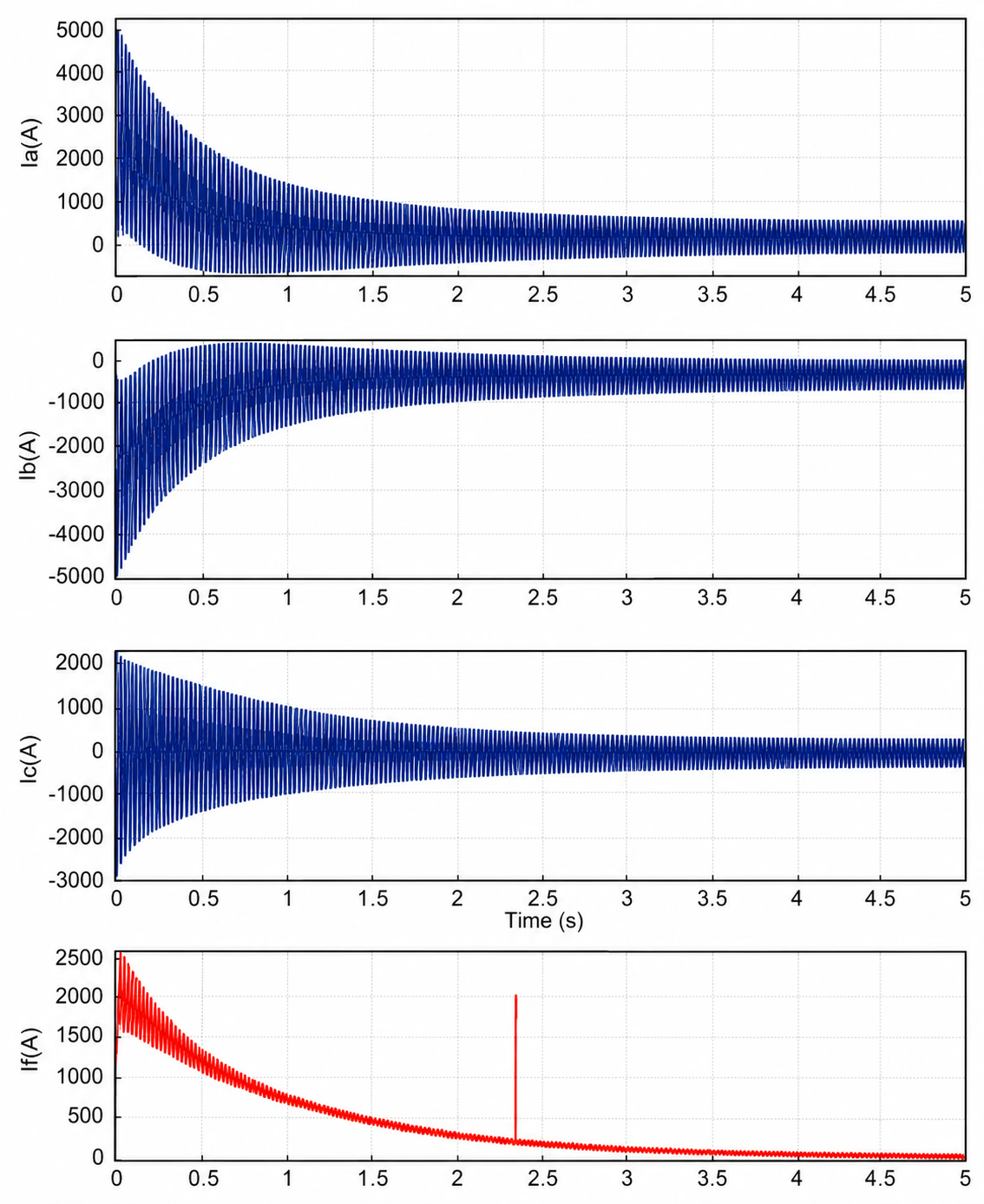
The sudden three-phase short-circuit response is one of the clearest ways to understand synchronous-machine characteristic parameters. Immediately after the fault, the armature current contains a high subtransient component, a slower transient component and a decaying DC offset. The field current also changes because the rotor circuits respond to the sudden change in stator current and air-gap flux. This measured response is the physical basis for interpreting \(X''_d\), \(X'_d\), \(X_d\), \(T''_d\), \(T'_d\) and the armature time constant.

IEEE Std 1110-2019 Figure 14: oscillograms of the armature phase currents and field current of a 361.4 MVA, 20 kV, two-pole turbine generator during a sudden three-phase short-circuit test, showing the decaying subtransient, transient and steady-state armature envelope and the field-current response. — **Figure 1 —** Armature and field currents following a sudden three-phase terminal short circuit. The armature-current envelope illustrates the subtransient, transient and steady-state periods, while the field-current response shows why rotor circuits are essential when interpreting synchronous-machine parameters.

Use this figure as a response-interpretation aid, not as a complete parameter-conversion method. A sudden three-phase short-circuit test mainly excites the direct-axis response. It is very useful for d-axis transient and subtransient parameters, but it does not fully determine the q-axis representation. Q-axis data, especially for round-rotor or solid-rotor machines, must be obtained from suitable tests, manufacturer calculations or frequency-response information.

Section 5

The three inductance levels in physical terms

Subtransient inductance

\(L''_d\) is the effective d-axis stator inductance immediately after a sudden disturbance, when the rotor circuit flux linkages cannot change instantaneously. The field and d-axis damper oppose sudden changes in their flux, and their induced currents make the machine appear to have a smaller effective inductance — hence a larger initial current. The q-axis has the analogous \(L''_q\) from the q-axis dampers. The subtransient inductance governs the initial fault-current peak, breaker duty, protection studies, generator terminal faults, the first-cycle torque and out-of-phase switching stress — it represents only the earliest part of the response and must not be used as a long-duration impedance.

Transient inductance

\(L'_d\) describes the machine after the fastest damper effects have decayed but before the field flux has fully adjusted; it is mainly the field-winding response, whose larger time constant outlasts the dampers. It lies between the subtransient and synchronous values (\(L''_d<L'_d<L_d\)) and controls the slower decay of the AC current after the first cycles — often more important than the subtransient value in voltage-recovery and stability studies, where the event lasts long enough for subtransient effects to decay. On the q-axis, a distinct transient inductance exists only if the rotor construction and the number of represented q-axis circuits support it; some salient-pole machines with a single q-axis damper move directly from subtransient to steady-state behaviour.

Synchronous inductance

\(L_d\) is the effective inductance after all transient rotor currents have decayed and the machine is in steady-state short circuit: dampers gone, field settled to the excitation condition, current limited by the synchronous reactance. It is the largest of the three, so the steady-state short-circuit current is normally the lowest part of the AC envelope. It is central to steady-state fault calculations and classical analysis, but it does not represent the initial duty on equipment right after a fault.

Section 6

Why damper windings control the first cycles

The dampers are short-circuited rotor circuits. When the stator flux changes suddenly, currents are induced in them that oppose the change and so lower the apparent stator impedance. Because damper circuits usually have small time constants compared with the field, their currents decay quickly — the rapid current decrement of the subtransient period. The d-axis damper shapes the d-axis subtransient response and the q-axis dampers the q-axis response; the number of damper circuits modelled sets how many distinct decay modes can be represented, but only if reliable data exists for them. A model with inadequate damper representation still runs in EMTP®, but it may under- or over-predict the initial fault current and torque.

Section 7

Why the field winding controls the slower transient period

The field winding is the main rotor excitation source. During a stator short circuit the armature reaction tends to demagnetise the rotor field, and the field circuit responds with currents that oppose the change in field flux linkage. Its time constant is larger than the dampers’, so its effect persists — which is why the transient period decays more slowly than the subtransient period. The d-axis transient time constant \(T'_d\) is closely tied to this field response, and its open-circuit and short-circuit versions differ because the stator boundary condition changes the effective magnetic circuit the field winding sees — a distinction that matters when converting manufacturer data into model parameters.

Section 8

Short-circuit and open-circuit time constants

Short-circuit time constants describe the decay of rotor-current components (and the AC envelope) with the stator short-circuited; open-circuit time constants describe the decay when the stator is open and a step is applied to the field voltage:

\[ T''_d \;<\; T'_d \qquad\qquad T''_q \;<\; T'_q \]

\(T''_d,\ T''_q\): d- and q-axis short-circuit subtransient time constants (damper decay)
\(T'_d,\ T'_q\): d- and q-axis short-circuit transient time constants (field / slower decay)

\[ T''_{d0} \;<\; T'_{d0} \qquad\qquad T''_{q0} \;<\; T'_{q0} \]

\(T''_{d0},\ T''_{q0}\): open-circuit subtransient time constants
\(T'_{d0},\ T'_{q0}\): open-circuit transient time constants

Open-circuit time constants are usually larger than the short-circuit ones, because the stator no longer provides the same short-circuit path for flux changes. The same rotor circuits are being observed under two different stator boundary conditions — which is precisely why a conversion is needed to recover the equivalent-circuit resistances and inductances. For some salient-pole models with one q-axis damper, \(T'_q\) / \(T'_{q0}\) may not be defined separately. A common error is to use open-circuit time constants where short-circuit values are required (or vice-versa) without conversion — it gives the wrong decay rates.

Section 9

The armature time constant and the DC offset

The DC component of the stator short-circuit current decays according to the armature time constant:

\[ T_a = \frac{L_2}{R_a} \qquad\qquad L_2 = \frac{L''_d + L''_q}{2} \]

\(T_a\): armature (DC-offset) time constant
\(L_2\): negative-sequence inductance
\(R_a\): armature resistance
\(L''_d,\ L''_q\): d- and q-axis subtransient inductances

The DC offset in the phases makes a magnetomotive-force pattern stationary relative to the stator, which the rotor sees as an alternating effect at synchronous frequency — so the effective inductance lies between \(L''_d\) and \(L''_q\), giving \(L_2\approx(L''_d+L''_q)/2\). The armature time constant governs DC-offset decay, asymmetrical fault current, breaker making duty and the peak fault current; the offset can dominate the first current peak even when the symmetrical AC current is well represented. The armature time constant is represented using an effective armature inductance and the stator resistance; that effective inductance is commonly associated with the subtransient or negative-sequence value, but the exact basis depends on the standard, data source and software convention, so the assumption used should be stated.

Section 10

Operational inductance — the frequency view

Machine behaviour can also be written with operational parameters in the Laplace domain, which show how the effective inductance changes with frequency:

\[ \psi_d(s) = G(s)\,v_F(s) + L_d(s)\,i_d(s) \qquad\qquad \psi_q(s) = L_q(s)\,i_q(s) \]

\(s\): Laplace-domain complex frequency variable (\(s=j\omega\) for a frequency response)
\(L_d(s),\ L_q(s)\): d- and q-axis operational (frequency-dependent) inductances
\(\psi_d(s),\ \psi_q(s)\): d- and q-axis flux linkages
\(i_d(s),\ i_q(s)\): d- and q-axis stator currents
\(G(s)\): armature-to-field transfer function
\(v_F(s)\): field voltage

\[ L_d(0) = L_d \;\;\xrightarrow[\text{slow}]{}\;\; L'_d \;\;\xrightarrow[\text{fast}]{}\;\; L''_d \qquad\qquad L_q(0) = L_q \]

At very low frequency the rotor circuits respond fully, so \(L_d(0)=L_d\); during slower transients the effective inductance is near \(L'_d\); during fast transients it approaches \(L''_d\). This is the unifying idea: the synchronous, transient and subtransient reactances are all correct — they are effective values for different parts of the response. Because an EMT waveform contains many frequencies, the effective machine impedance the network sees depends on the time scale: a slow disturbance sees a different machine from a fast one.

Armature-to-field transfer function

\(G(s)\) describes how a field-voltage change affects the d-axis armature flux. Its gain falls with frequency: low-frequency excitation changes influence terminal voltage and internal flux, but fast field-voltage variations are filtered by the machine’s electromagnetic dynamics, and very fast terminal transients are not controlled by the excitation system at all. This avoids a common misconception — increasing field voltage does not control the first microseconds or first few electrical degrees of a fast transient. On the q-axis there is no field, so \(L_q(s)\) is governed by the dampers and rotor construction; a round-rotor machine may need more detailed q-axis representation because solid-rotor eddy-current paths act like extra dampers.

Section 11

Model structures and number of damper circuits

Models differ in how many d- and q-axis rotor circuits they carry. A simple d-axis model has only the field circuit; a fuller one adds one or two d-axis dampers. The q-axis may have zero, one, two or three dampers depending on the required accuracy and the available data — combinations often summarised as a model structure naming the number of d- and q-axis circuits. The choice depends on rotor construction, available data, the transient frequency range, the study objective, and whether subtransient behaviour, torsional damping or measured frequency response must be matched. A laminated salient-pole machine does not need the same q-axis representation as a solid round-rotor machine, whose solid rotor provides eddy-current paths that behave like extra damper circuits — so round-rotor machines often need more detailed q-axis modelling.

Section 12

When a complex model is not justified

A more complex model is not automatically better: more rotor circuits need more parameters, and if those are not available they must be estimated — introducing uncertainty that can outweigh the benefit. Adding a second q-axis damper may improve a frequency-response match, but with no data to fix that branch the model only looks more accurate.

The rule

Use the simplest model that captures the physical behaviour controlling the study result, and do not add internal branches that the data cannot support. Close-up fault current needs subtransient parameters; long-duration stability leans on transient and synchronous behaviour; subsynchronous resonance needs a carefully chosen d- and q-axis model; and high-frequency surge studies may not be controlled by these low-frequency rotor circuits at all.

Section 13

From characteristic data to model parameters

The characteristic reactances and time constants on this page are not the final internal branch parameters. Before an EMTP® simulation they must be converted into the stator, field and damper resistances, leakage inductances and mutual inductances of the equivalent circuit. That conversion depends on the chosen model order, the stator-leakage assumption, the time-constant type (open- or short-circuit) and the saturation basis, and inconsistent input data can yield a non-physical result such as a negative leakage inductance. The detailed procedure — including operational-inductance fitting and the Canay characteristic inductance — is on the next data-conversion page.

Four kinds of “parameter”

Keep them distinct: characteristic data (a data-sheet reactance describing machine response), converted equivalent-circuit branch parameters (internal leakage/mutual inductances and resistances), EMTP® input parameters (what the model interface actually asks for), and the program’s internal numerical state variables. A data-sheet reactance is not automatically the same as an internal branch — EMTP® may ask for characteristic quantities or for converted branch quantities depending on the model interface, so the required input form must be checked.

Section 14

Reading the reactances

Read in reactance terms (recall \(X=\omega L\)), the three d-axis levels mirror the inductance levels described above: \(X_d\) is the steady-state response, \(X'_d\) the transient response and \(X''_d\) the initial subtransient response. The same reading applies to the q-axis, where \(X''_q\) is the initial response and \(X'_q\) is defined only where the q-axis rotor detail supports it:

\[ X''_d < X'_d < X_d \qquad\qquad X''_q < X'_q < X_q \]

If the ordering is not satisfied, check the data: a base error, a saturated/unsaturated mismatch, a sign-convention issue or an inappropriate parameter source. For some laminated salient-pole machines the q-axis is represented with only one damper, so it may not distinguish q-axis transient and steady-state behaviour the way the d-axis does — the available data and machine type must be considered.

Note — Do not infer a complete q-axis model only from a three-phase sudden-short-circuit trace. The q-axis is poorly excited in this test, so \(X'_q\), \(X''_q\), \(T'_q\) and \(T''_q\) should only be used when they are supported by suitable test data, manufacturer calculation or a justified model structure.

Section 15

Saturated and unsaturated parameters

Parameters may be given as saturated or unsaturated values, and the distinction matters. Unsaturated reactances come from the air-gap line or the low-flux region of the magnetisation curve; saturated reactances reflect operation at a specified voltage or flux where the iron is already partly saturated. The difference can be significant, especially for \(X_d\). If saturated and unsaturated data are mixed without care, the equivalent circuit will not reproduce the intended operating condition — so for load-rejection, overvoltage or excitation-response studies the saturation curve and the parameter basis should be stated explicitly.

Section 16

Practical checks on machine parameters

Before using the model, confirm:

The MVA base, the line-to-line RMS voltage base, the frequency base and the pole count are all correct; the armature resistance is on the correct base.
The d- and (where applicable) q-axis reactance orderings are physically reasonable; all transient and subtransient time constants are positive.
Open-circuit time constants are not accidentally used as short-circuit values, or vice-versa; saturated and unsaturated data are not mixed unintentionally.
The derived equivalent-circuit resistances and inductances are positive and physically meaningful.
The initial fault current roughly matches the value expected from \(X''_d\); the later envelope follows the transient and steady-state values; the DC-offset decay is consistent with \(T_a\).
The field-current and electromagnetic-torque responses are physically plausible.
The model stays stable in a no-disturbance run.

These checks are necessary, not optional — a machine model with wrong internal parameters can still converge numerically.

Section 17

Common modelling mistakes

Avoid these

Using \(X_d\) or \(X'_d\) instead of \(X''_d\) for first-cycle (subtransient) duty.
Confusing open-circuit and short-circuit time constants.
Mixing saturated and unsaturated reactances, especially for \(X_d\).
Mixing machine-base and system-base per-unit values.
Ignoring the DC offset when checking the first current peak.
Assuming a meaningful q-axis transient (\(X'_q\)) exists for every machine.
Building a higher-order rotor model than the available data supports.
Treating manufacturer reactances and time constants as the final internal branch parameters.
Omitting q-axis damper detail where torque or damping matters (notably round-rotor machines).
Trusting a converged simulation without checking the physical response.

Section 18

Where this fits in the series

This guide explains the characteristic reactances and time constants that populate the per-unit equivalent circuits introduced on the previous page, Per-Unit Representation and Equivalent Circuits. The next page, Data Conversion Procedures, explains how these characteristic quantities are converted into the internal stator, field and damper parameters the EMTP® model requires; the test-procedure and magnetic-saturation pages then cover how the data is measured and how saturation is represented.

Section 19

Suggested report wording

Model statement — for a study report

“The synchronous-machine parameters were interpreted from the manufacturer/test characteristic data, including the synchronous, transient and subtransient reactances, the relevant open- and short-circuit time constants, armature resistance and saturation basis. The sudden three-phase short-circuit response was used as the reference behaviour: subtransient current dominated by the damper circuits, transient current governed mainly by the field winding, steady-state current limited by the synchronous reactance, and a decaying DC offset represented by the armature time constant. The selected d- and q-axis data were checked for base consistency, reactance ordering, time-constant type, saturation basis, plausible current envelope, field-current behaviour, torque response and stable no-disturbance initialisation before being used in the EMTP® study.”

Section 20

Main takeaway

Parameters are physical decay paths, not just numbers to type in

Synchronous-machine reactances and time constants are not isolated data-sheet numbers — they describe the physical short-circuit response of the machine. \(X''_d\) and the damper circuits define the first cycles, \(X'_d\) and the field circuit define the slower transient period, \(X_d\) defines the final steady-state current, and \(T_a\) controls the DC-offset decay. The message: a reliable EMTP® model needs these quantities on the correct base, with the correct saturation and time-constant convention, and validated against the expected current, field and torque response.

References

The reference text for the derivation, the IEEE/IEC test-procedure standards that define these parameters, and the standard machine-modelling works.

J. A. Martínez-Velasco, Ed., Power System Transients: Parameter Determination, Ch. 5 (Synchronous Machines). Boca Raton, FL, USA: CRC Press, 2010.
IEEE Std 115-2009, IEEE Guide for Test Procedures for Synchronous Machines. New York, NY, USA: IEEE.
IEC 60034-4, Rotating Electrical Machines – Part 4: Methods for Determining Synchronous Machine Quantities from Tests. Geneva, Switzerland: International Electrotechnical Commission.
IEEE Std 1110-2019 (Revision of IEEE Std 1110-2002), IEEE Guide for Synchronous Generator Modeling Practices and Parameter Verification with Applications in Power System Stability Analyses. Piscataway, NJ, USA: IEEE, 2020.
P. Kundur, Power System Stability and Control. New York, NY, USA: McGraw-Hill, 1994.
P. M. Anderson and A. A. Fouad, Power System Control and Stability, 2nd ed. Piscataway, NJ, USA: IEEE Press / Wiley, 2003.

Part Five Reading now

Parameters and Short-Circuit Response

The meaning of the characteristic reactances and time constants, and the subtransient, transient and steady-state periods of the short-circuit current with its DC offset.

Series progress 5 of 9

Part Six

Data Conversion Procedures

Converting manufacturer and test data into the fundamental equivalent-circuit parameters — operational inductances, model order, Canay’s characteristic inductance and validation.