Renewable Modelling · Control Interactions & Model Selection

IBG Control Interactions, SSCI and Choosing the Right Model

Fast, high-gain converter controllers do not act in isolation: they interact with each other, with HVDC ties and FACTS devices, and with series-compensated lines — and in a weak grid those interactions can turn into sustained oscillations. This page builds on the RMS and EMT modelling foundations and explains the interaction phenomena that decide when detailed EMT or impedance-based analysis becomes necessary. It sorts the three sub-synchronous interactions, shows why control interaction (SSCI) needs no rotating mass, looks at the roughly 50% penetration turning point that probabilistic studies keep finding, and — the practical payoff — sets out how to choose between an RMS and an EMT model for each kind of study, drawing on the frequency-stability, voltage-deviation and small-signal / islanding guides.

Reading time ≈ 32 min · Interactions, SSCI, penetration & model choice

This is the final guide, and it brings the series together. Building on every page before it — the IBG characteristics, the inverter, the RMS / phasor and EMT models, and the frequency, voltage, small-signal and islanding studies — it uses all of them to explain the converter interaction phenomena that decide when detailed EMT, impedance-based analysis or EMT validation becomes necessary. A converter’s controls are fast and high-gain, and once several of them — plus HVDC ties and FACTS devices — sit electrically close together, they stop behaving independently. They interact, and in a weak grid that interaction can grow into a sustained oscillation. The earlier guides told you how to build an inverter-based-generation (IBG) model; this one closes the series by explaining what can go wrong when many fast models are connected — control interaction, SSCI and impedance-based stability — and how to make the final choice between RMS, EMT and impedance-based analysis.

Where this sits in the series
  • The inverter-characteristics guide explained the inverter itself — its controls, protection and capability functions.
  • The RMS-models guide explained how IBGs are simplified inside RMS / phasor models.
  • The EMT-models guide explained EMT models and why fast waveform and control phenomena need more detail.
  • This page now explains what can go wrong when fast IBG controls interact with the grid, with HVDC, FACTS devices, series capacitors or neighbouring converters — and how to choose the right model for each study.
By the end of this page, you should understand
  • what a control interaction is, and why converter controllers can become unstable even when each device is stable on its own;
  • why weak grids increase interaction risk;
  • the difference between SSR, SSTI and SSCI, and why SSCI needs no turbine shaft;
  • why SSCI is especially relevant for IBG, Type-3 / Type-4 wind, PV and battery storage;
  • what impedance-based stability analysis is, and why Nyquist and Bode plots are used;
  • what probabilistic / Monte Carlo stability assessment means;
  • and how to choose between RMS and EMT for different study types.
Abbreviations used on this page
IBGInverter-based generation (or generator)
RMSRoot-mean-square (phasor) simulation
EMTElectromagnetic transient (time domain)
EMTP®Electromagnetic Transients Program (an EMT tool)
HVDCHigh-voltage direct current
FACTSFlexible AC transmission systems
SVCStatic VAr compensator
STATCOMStatic synchronous compensator
WPPWind power plant
WTGWind-turbine generator
DFIGDoubly-fed induction generator (Type-3 wind)
PVPhotovoltaic
BESSBattery energy storage system
VSCVoltage-source converter
LCCLine-commutated converter
PLLPhase-locked loop
SCRShort-circuit ratio (grid strength)
SSRSub-synchronous resonance
SSTISub-synchronous torsional interaction
SSCISub-synchronous control interaction
PODPower oscillation damping
FRTFault ride-through
LVRT / HVRTLow- / high-voltage ride-through
PCCPoint of common coupling
POIPoint of interconnection
Key idea
  1. A control interaction is a system problem: fast, high-gain converter controllers couple through the grid impedance, and a set of devices each stable alone can be unstable together. The risk grows in weak grids (low SCR) and when nearby devices share the same voltage.
  2. The tool is impedance-based stability analysis: represent the converter and the grid as frequency-dependent impedances and test the combined loop with Nyquist and Bode — because a device that looks fine at 50 Hz can create negative damping at a control-loop frequency.
  3. Sub-synchronous interaction has three forms — SSR (machine ↔ series capacitor), SSTI (machine shaft ↔ HVDC/SVC control) and SSCI (converter control ↔ network). SSCI needs no rotating mass, which is why it is the IBG-era problem.
  4. Choose the model by the phenomenon, not the technology: RMS for wide-area screening and probabilistic studies, EMT and impedance-based analysis for SSCI, weak-grid interaction, harmonic resonance and fast protection — and benchmark RMS against EMT where it matters.
Key terms used on this page
01Control interaction
Adverse coupling between the fast controllers of nearby power-electronic devices, so their combined feedback response oscillates or grows.
02Control instability
An oscillation created or amplified by the control loops — growing voltage, current, power, dc-link or PLL-angle oscillation, or a converter trip.
03Weak AC grid
Low short-circuit power relative to the converter rating (low SCR); high voltage-angle sensitivity and strong converter–grid coupling.
04Impedance-based stability
Representing the converter and grid as frequency-dependent impedances and testing whether their combined loop is stable and well damped.
05Bode plot
Gain and phase versus frequency — used to spot frequencies where the converter–grid loop has high gain and dangerous phase shift.
06Nyquist criterion
A frequency-domain test of whether the open-loop response predicts a stable or unstable (growing) closed loop.
07Impedance scan
Measuring the converter or network impedance across frequency (by injection and response) to build the impedance model used above.
08SSR / SSTI / SSCI
Sub-synchronous resonance / torsional interaction / control interaction — the three sub-synchronous phenomena compared in Section 3.
09Monte Carlo assessment
Running many dynamic simulations over randomly sampled conditions to get a distribution of outcomes, not a single answer.
10Frequency nadir
The lowest frequency reached after a disturbance; set by inertia and the speed of the active-power (frequency) response.
11Grid-following
A converter that uses a PLL to synchronise to and follow an existing grid voltage.
12Grid-forming
A converter that establishes voltage magnitude and frequency more like a voltage source; helps weak grids but still needs interaction studies.

Section 1

What a control interaction is

Start with a plain definition. A control interaction occurs when two or more control systems influence the same voltage, current, power or frequency signal, and their combined feedback response creates oscillation, amplification or instability. The crucial and counter-intuitive part follows: each controller may be perfectly stable when tested alone, yet the combined system can become unstable once the devices are connected through the grid impedance. This is why a control interaction is a system problem, not a single-device problem.

Why are IBGs more interaction-prone than synchronous machines? Because their response is mostly software. An IBG’s behaviour is shaped by its PLL, its current controller, its active- and reactive-power controllers, its current limiter and its protection logic — and those controls can react in milliseconds. If several fast controllers respond to the same bus voltage or current, they can effectively fight one another. A synchronous machine, by contrast, has physical inertia and electromagnetic dynamics that set its response; an IBG’s response is defined by control code within its current and energy limits.

The weak grid is where this turns dangerous, and the mechanism is a feedback loop worth tracing slowly:

  • A strong grid behaves like a stiff voltage source — the converter’s current has little effect on the voltage magnitude and angle.
  • A weak grid has higher impedance — the converter’s current strongly changes the local voltage and angle.
  • The converter measures that disturbed voltage (through its PLL) and reacts again through its current controller.
  • That closes a feedback loop between the converter and the grid impedance.

Follow the chain once: converter current injection → voltage drop across the grid impedance → changed PCC voltage magnitude and angle → PLL and controller response → changed current injection — and back to the start. If the phase delay and gain around this loop are unfavourable, the response grows instead of decaying. A low SCR increases the chance of exactly that. As on the earlier pages, treat SCR thresholds as warning signs, not universal pass/fail limits.

IBG control interaction feedback loop An IBG converter injects current into the point of common coupling (PCC). The current flows through the grid impedance to the AC grid, so it changes the PCC voltage. The converter’s PLL and current controller measure that voltage and adjust the injected current, closing a feedback loop. A nearby HVDC, STATCOM, SVC or other IBG is connected to the same PCC and takes part in the same loop. PCC busbar Z grid AC grid (stiff voltage source) IBG converter current controller PLL · current limiter injected current I measured PCC voltage → PLL Nearby HVDC / STATCOM / SVC / other IBG
Figure 1 — The control-interaction feedback loop. The converter injects current into the PCC; that current, flowing through the grid impedance, changes the PCC voltage; the PLL and current controller measure the change and adjust the injection — a closed loop. A nearby HVDC, STATCOM, SVC or IBG on the same busbar joins the same loop, so the devices must be studied together.
Grid-following versus grid-forming

Two converter families sit behind this. A grid-following converter uses a PLL (or equivalent) to synchronise to and follow an existing grid voltage — it is the loop drawn above, and it is the more interaction-prone on a weak grid. A grid-forming converter establishes voltage magnitude and frequency more like a voltage source, which can improve weak-grid operation. Grid-forming control is not a magic cure, though: it still requires careful interaction studies of its own, so do not assume it removes every stability concern.

Section 2

Impedance-based stability analysis

How do you test a loop like Figure 1 before it bites you on site? The standard tool is impedance-based stability analysis, and the idea is more intuitive than the mathematics that surrounds it.

  • The converter can be represented by an output impedance (or admittance) over frequency.
  • The grid can be represented by an equivalent impedance over frequency.
  • Stability depends on how these two frequency-dependent behaviours interact.
  • The method checks whether the combined converter–grid loop has enough damping and phase margin.

The phrase frequency-dependent impedance is the heart of it: the apparent resistance and reactance of a converter or a network change with frequency. A device may look perfectly well behaved at 50 Hz, yet create negative damping or a resonance at a sub-synchronous, harmonic or control-loop frequency. That is precisely why a normal load-flow or short-circuit result — both fundamental-frequency snapshots — is not enough to rule out an interaction.

Two frequency-domain plots do the judging, and neither needs its full control-theory proof to be useful here:

  • A Bode plot shows gain and phase versus frequency. It helps identify the frequencies where the converter–grid loop has high gain and a dangerous phase shift.
  • A Nyquist analysis checks whether the open-loop frequency response predicts a stable or an unstable closed-loop system. The teaching message is not the mathematical proof; it is that Nyquist tells you whether the converter and grid impedance together create a growing oscillation.

The impedance data itself comes from an impedance scan — injecting a small signal across frequency and measuring the response, in a time-domain EMT run or a dedicated tool. Our frequency-scan, time-domain impedance-scan and grid-side-scan guides work through the method in detail.

A caution on impedance scans

Impedance-based analysis is powerful, but the result is only as good as its assumptions. It depends on the operating point, the control mode, the PLL settings, the current limiters, the network equivalent, the measurement method, and whether the model is single-input/single-output or the fuller multi-input/multi-output form. Change any of these and the impedance — and the stability verdict — can change with it. Treat a single scan as one operating condition, not a guarantee.

One more mechanism deserves naming, because it is where interactions most often start: a shared input signal. If several devices regulate the same voltage, they may all inject or absorb reactive current at the same time; one device’s action changes the voltage the others see; and their controllers can then unintentionally amplify one another. This is exactly why nearby IBG, a neighbouring wind power plant (WPP), HVDC, STATCOM and SVC models must be studied together, not one at a time. These interactions echo the classic line-commutated-converter (LCC) HVDC and SVC control interactions long studied by CIGRE (WG 14.28) and the wind-plus-power-electronics interactions of CIGRE B4.62 (TB 671), which is a key reference for weak-AC-network connection of wind farms; the impedance-based stability criterion for grid-connected inverters is widely associated with the work of J. Sun.

Section 3

Sub-synchronous interaction: SSR, SSTI and SSCI

First, the word. Sub-synchronous means below the fundamental system frequency: below 50 Hz on a UK / European system, and below 60 Hz on a North American one. These frequencies can still be electrically dangerous, because the controls and the network resonances may amplify them rather than damp them.

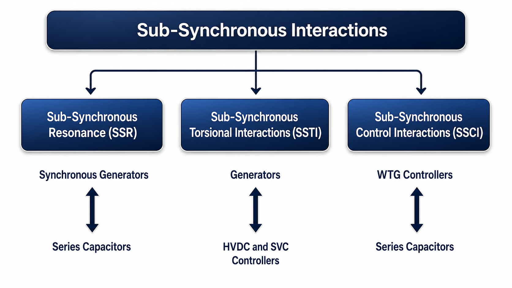
Series capacitors are often the trigger, so it is worth knowing why. Series capacitors compensate a line’s reactance and improve its transfer capability — but they also create an electrical resonant frequency with the network inductance, and that resonance usually sits in the sub-synchronous range. It is that resonance which can interact with a synchronous-machine shaft or with a converter’s controls. With that in place, the three sub-synchronous phenomena separate cleanly (Figure 2):

  • SSR (sub-synchronous resonance) — interaction between a synchronous generator’s shaft system and a series-compensated electrical network.
  • SSTI (sub-synchronous torsional interaction) — interaction between a turbine-generator’s torsional shaft mode and a power-electronic controller such as HVDC or SVC.
  • SSCI (sub-synchronous control interaction) — interaction between a converter control system and the electrical network, often involving series capacitors or weak-grid impedance, without requiring a turbine shaft mode.
Classification of sub-synchronous interactions: a top box, Sub-Synchronous Interactions, branches into three — Sub-Synchronous Resonance (SSR) between synchronous generators and series capacitors; Sub-Synchronous Torsional Interactions (SSTI) between generators and HVDC and SVC controllers; and Sub-Synchronous Control Interactions (SSCI) between WTG controllers and series capacitors.
Figure 2 — The three sub-synchronous interactions. SSR couples synchronous generators to series capacitors; SSTI couples generators to HVDC and SVC controllers; SSCI couples WTG (converter) controllers to series capacitors.

The clearest way to hold the three apart is side by side:

Table 1 — SSR, SSTI and SSCI compared.
InteractionMain equipment involvedMechanical shaft required?Typical triggerMain modelling toolMain risk
SSRSynchronous generator + series capacitorsYesSeries compensation of the lineEMT (with shaft model)Shaft fatigue and failure
SSTITurbine-generator shaft + HVDC / SVC controlYesHVDC or SVC controller nearbyEMT (with shaft model)Shaft torsional fatigue
SSCIConverter control + network / series capacitorsNo — no rotating mass neededConverter on a series-compensated or weak gridEMT and impedance-based analysisGrowing electrical oscillation, over-voltage, control / converter damage
SSR, SSTI and SSCI mechanisms compared Three mini diagrams. SSR: a synchronous generator with a mechanical shaft interacts with a series capacitor and network resonance. SSTI: a synchronous generator shaft interacts with an HVDC or SVC controller. SSCI: a converter controller interacts with the grid and series-capacitor impedance, with no mechanical shaft. SSR SSTI SSCI G machine + shaft C ser series cap resonance G machine + shaft HVDC /SVC ctrl torsional convertercontrol grid /C ser no shaft required control interaction
Figure 3 — The three mechanisms side by side. SSR and SSTI both need a mechanical shaft; SSCI is purely between the converter control and the network impedance, with no rotating mass required — which is why it is the interaction of the IBG era.

SSR and SSTI act on the generator shafts and, in severe cases, cause shaft fatigue and failure. SSCI is important for IBGs precisely because the converter controller — typically a voltage-source converter (VSC) — is the dynamic element. The instability can occur even with no large synchronous-generator shaft anywhere nearby, which makes PV, Type-3 wind (DFIG), Type-4 (full-converter) wind, battery storage (BESS), HVDC and STATCOM-dominated areas more exposed to control-interaction problems. Type-3 and Type-4 wind behave differently — the DFIG’s stator is directly connected while only its rotor is converter-fed, whereas a Type-4 machine is fully decoupled by its converter — so the two should not be treated as identical in an SSCI study. It is most pronounced at low SCR and when the devices are electrically close or on the same busbar. The frequency-scan and impedance-based methods for finding it are covered in the time-domain impedance scan, grid-side scan and turbine-side and verification guides.

Section 4

Modelling an interaction study

A control-interaction study is, at heart, a small-signal analysis around the operating point — so, as in small-signal stability, the model needs the full control and capability set but not the protections and limiters, because they do not act for such small signals. That maps straight onto the Control / Protection / Capability classes from the inverter-characteristics guide. Table 2 states it in its simplest form.

Table 2 — Necessary IBG functionalities for a controller-interaction study (after CIGRE Table 3.11).
CategoryFunctionalitiesModel?Note
ControlAll control functionsYesthe interaction lives in the controls
ProtectionAll protection functionsNothey do not act for small signals
CapabilityAll capability functionsYesthey shape the small-signal response

When you run the study, the useful outputs to plot — the signals that reveal an interaction — are the PCC voltage magnitude and angle; the converter current magnitude and its dq components; the active and reactive power; the PLL frequency and angle; the dc-link voltage if available; the current-limiter status; the protection flags; the outputs of nearby STATCOM, HVDC or SVC devices; and, where applicable, the frequency spectrum or the modal damping. Where a known mode must be damped, a power oscillation damping (POD) controller can be added — but it must itself be checked for new interactions.

Practical study checklist — before a control-interaction / SSCI study
  • Is the grid weak at the POI / PCC (low SCR)?
  • Are there series capacitors, filters, long cables or tuned shunts nearby?
  • Are multiple converters, HVDC links, SVCs or STATCOMs electrically close?
  • Do several devices regulate the same voltage or reactive power?
  • Are the vendor control modes and PLL settings known?
  • Are the current limits and protection models included?
  • Is a frequency-dependent network model needed?
  • Is the RMS model validated for this operating condition?
  • Is EMT or impedance scanning required?

Section 5

How much IBG can a system carry?

As IBG displaces synchronous machines, one of the newer planning questions is the maximum penetration — or, equivalently, the minimum synchronous generation that must stay connected to keep the system stable. First, define the term. IBG penetration is the share of generation or power supply provided by inverter-based resources at a given time or in a given study case. It can be measured several ways — as a percentage of instantaneous generation, of load served, or of installed capacity — and these are not the same number; this page uses instantaneous generation share unless stated otherwise.

IBGs change stability in two ways: they shift the pre-disturbance operating point, and they behave differently during and after disturbances. Their intermittency adds uncertainty to the pre-fault state, which raises the need to evaluate worst-case conditions — and that points to a probabilistic stability assessment rather than a single deterministic case.

Monte Carlo / probabilistic assessment, in plain terms

A deterministic study checks one selected case. A probabilistic study checks many possible cases. In a Monte Carlo simulation, uncertain inputs — load level, renewable output, fault location, fault-clearing time, dispatch — are randomly sampled many times, and the result is not one stability answer but a probability or distribution of outcomes.

A probabilistic-assessment workflow
  • 1. Select the uncertain variables.
  • 2. Define probability distributions or sampling ranges for them.
  • 3. Create many operating cases by sampling.
  • 4. Run RMS (or EMT) simulations across the cases.
  • 5. Record stability indicators — frequency nadir, damping, voltage recovery, loss of synchronism.
  • 6. Identify the risk level and the critical conditions.

These studies keep finding a turning point around 50% penetration: from a transient-stability view the system tends to become more stable as IBG rises up to about 50%, then more stressed beyond it; from a frequency view the frequency nadir stays tightly grouped until about 50%, then scatters. But a word of caution: the frequency nadir is the lowest frequency reached after a disturbance, set by the inertia and the speed of the active-power response — and more IBG does not automatically mean a worse nadir if the IBG provides fast frequency response, headroom or storage. Likewise, do not use 50% as a planning rule without repeating the study for the actual network: it is a study-specific observation, not a universal limit, and the real limit depends on network strength, dispatch, inertia, protection, converter controls, the grid-forming / grid-following mix, fault locations, the load model and the operating condition (Ireland, for instance, has operated safely above 50%). The operational lesson is to focus on the minimum share of synchronous generation the system actually needs.

Section 6

Choosing RMS or EMT

Every model has limits, so the model type must follow the objective of the study. The most important rule first: do not choose RMS or EMT just because the plant is PV, wind or BESS. Choose the model based on the phenomenon, the time scale, the grid strength, the control-interaction risk, the protection behaviour and the required outputs. Table 3 gives the usual mapping.

Table 3 — Choosing between RMS and EMT models by study type (after CIGRE Table 3.12).
Study typeRMS normally acceptable?EMT required whenKey IBG functions to represent
Frequency stabilityYesrarelyP(f), fast frequency response, inertia emulation
Transient / rotor-angle stabilityYes (validated)large plant on a very weak gridFRT, current limit, P/Q control
Large voltage deviation / FRTFor bulk screeningdetailed ride-through near zero voltageLVRT / HVRT, current limiter, protection
Short-circuit current contributionNoalmost alwayscurrent limit, PLL, protection
Small-signal stabilityYesweak grid / fast controlsfull control & capability set
SSCI / control interactionNoalwaysinner current loop, PLL, series-cap network
Harmonic resonanceNoalwaysconverter impedance vs frequency
Unintentional islandingYesanti-islanding uses voltage harmonicsanti-islanding, protection
Protection coordinationSometimeswaveform-dependent protectionprotection, current limit
Long-term voltage stabilityYesrarelyV/Q control, reactive capability

The choice connects straight back to the earlier pages: from the inverter-characteristics guide, include the relevant Control, Protection and Capability functions; from the RMS-models guide, use RMS when phasor-domain behaviour is enough; from the EMT-models guide, use EMT when the waveform, fast control, switching, unbalance or weak-grid interaction determines the result.

Why can RMS miss a control interaction in the first place? Because RMS models often remove or simplify the inner current loops, the detailed PLL behaviour, the switching effects and the fast protection. Those simplifications are perfectly acceptable for many bulk stability studies, but they can hide the exact mechanism of a converter–grid control instability. So in weak-grid or SSCI studies, RMS results should be benchmarked against EMT or impedance-based analysis.

None of which makes the page anti-RMS — quite the opposite. RMS remains extremely valuable for screening many cases, identifying stressed operating points, testing broad dispatch scenarios and running the probabilistic studies of Section 5. EMT is then used for the selected critical cases where the detailed behaviour matters. The two are partners, and a sensible study uses them in that order.

Choosing RMS or EMT — a decision workflow A left-to-right flow. Start from the study objective, then the time scale and phenomenon, then check grid strength and nearby converters, FACTS or HVDC. A decision splits into RMS screening for slow, strong-grid phenomena, or EMT and impedance-based analysis for fast, weak-grid or control-interaction phenomena. Both lead to validation against vendor data or measurements. Study objective Time scale &phenomenon Grid strength &nearby converters RMS screeningslow / strong-grid EMT / impedancefast / weak-grid / SSCI Validate vs vendor data / measurements
Figure 4 — A recommended workflow. Start from the objective, identify the phenomenon and time scale, then check grid strength and nearby power-electronic devices; run RMS screening for slow, strong-grid cases and EMT or impedance-based analysis for the fast, weak-grid or control-interaction cases — and validate the result against vendor data or measurements.

Put together, the recommended sequence is: start from the study objective; identify the phenomenon and time scale; check the grid strength and nearby power-electronic devices; decide whether a control interaction is plausible; run RMS screening if appropriate; run an EMT or impedance-based study for the critical weak-grid / control-interaction cases; check the protection, current limits and operating-mode changes; and validate against vendor data or measurements.

Section 7

Common mistakes

The traps that most often catch a control-interaction or SSCI study — each a theme from the sections above:

Eight traps to avoid
  • Treating 50% IBG penetration as a universal limit instead of a study-specific result.
  • Using RMS for SSCI without EMT or impedance-based validation.
  • Studying each converter / STATCOM / HVDC device separately when they share the same bus voltage.
  • Forgetting the PLL and current-limiter effects in weak-grid studies.
  • Ignoring series-capacitor resonance.
  • Assuming a stable individual device guarantees a stable combined system.
  • Using generic converter models for project-specific control-interaction work.
  • Ignoring protection and operating-mode changes during disturbances.

Key points

Key points

Control interaction is a system problem, not a single-device problem

A converter, STATCOM, SVC or HVDC link can be perfectly stable on its own yet unstable once connected to a weak grid or to other fast controllers. RMS is excellent for wide-area screening and probabilistic studies, but SSCI, weak-grid converter interaction, harmonic resonance and fast protection behaviour normally require EMT, impedance-based analysis, or both. The recurring craft is to model the functionalities the specific study needs — the Control, Protection and Capability classes from the inverter-characteristics guide — choose RMS or an EMT tool such as EMTP® to match the phenomenon, benchmark the two where the grid is weak, and remember that IBGs cannot do everything a synchronous machine does — so the real planning target is the minimum synchronous generation the system must keep. For the machine-versus-inverter foundations, see the characteristics of IBG guide.

References

References

The CIGRE/CIRED joint working-group brochure on inverter-based generation is the primary reference; CIGRE Technical Brochure 671 covers wind-plant connection to weak AC networks and the associated control interactions; and the impedance-based stability criterion underpins the frequency-domain interaction analysis.

  1. CIGRE/CIRED Joint Working Group, Modelling of Inverter-Based Generation for Power System Dynamic Studies. CIGRE Technical Brochure.
  2. CIGRE Working Group B4.62, Connection of Wind Farms to Weak AC Networks. CIGRE Technical Brochure 671.
  3. J. Sun, “Impedance-Based Stability Criterion for Grid-Connected Inverters,” IEEE Transactions on Power Electronics, vol. 26, no. 11, pp. 3075–3078, 2011.

Twelve-Part Technical Series

Modelling Inverter-Based Generation

A twelve-part guide to modelling inverter-based generation — from device characteristics and the RMS and EMT model families, through model adequacy, validation and large-scale wide-area EMT, to frequency, voltage and small-signal stability studies.

Part 12 Reading now

Control Interactions, SSCI and Model Selection

The capstone: converter-grid interaction, SSCI, impedance-based stability and the final RMS / EMT / impedance choice.

Series progress 12 of 12