Electromagnetic Transient Studies

Transformer Modelling in EMTP® — High-Frequency Models

At high frequency the winding ceases to be a lumped inductance and behaves as a distributed network in which capacitances and travelling waves dominate. This part covers terminal and internal models, the MTL/STL/ladder winding representations, capacitive voltage transfer, and how EMTP® extends beyond the BCTRAN validity range with added capacitances and a Frequency-Dependent Branch.

Reading time ≈ 11 min · Part Three of the series

At high frequency the transformer no longer behaves mainly as a leakage impedance and a magnetising branch. The winding becomes a distributed electrical network of inductances, resistances and capacitances. High-frequency studies must therefore consider capacitance to ground, capacitance between windings, inter-turn capacitance, travelling-wave behaviour, damping and possible winding resonance.

High-frequency modelling becomes necessary only when the objective moves beyond power-frequency behaviour, inrush and saturation. It is triggered when the applied voltage carries fast-front or resonant content capable of exciting winding capacitances, terminal-to-terminal voltage transfer, winding resonances or internal insulation stress — at which point the question shifts from what the terminals carry to where the insulation is stressed.

This page focuses on transformer models for fast-front and very-fast-front transients — lightning surges, steep switching surges, cable–transformer interactions and transferred overvoltages between windings.

Key takeaway

At high frequency, capacitances and distributed winding behaviour dominate the response — not the core.
A terminal model is enough when only external terminal voltages and currents are needed.
An internal winding model is required to calculate inter-turn, inter-disc or internal insulation stress.
High-frequency voltage transfer between windings does not follow the turns ratio — it follows the capacitance network.

When a winding is exposed to a steep voltage wave — a lightning surge entering through the line, a switching surge from a breaker, a cable-energisation front, a restrike or a disconnector operation — the transformer can no longer be treated as the lumped magnetic circuit used for low-frequency studies. Two facts drive everything in this section:

The stress depends on the rate-of-rise, not only on the peak. A low-amplitude but very steep front can be more dangerous than a higher, slower one, because at the first instant the impressed voltage does not distribute uniformly along the winding. The leading edge is dropped almost entirely across the first turns/discs nearest the energised terminal, producing a strongly non-uniform initial distribution and large turn-to-turn stresses that never appear in a power-frequency analysis.

The winding is a distributed network, not a single inductance. Series inductance, conductor (skin/proximity) resistance, turn-to-turn capacitance, winding-to-ground and winding-to-winding capacitance, and dielectric losses all act together; surges propagate along the winding as travelling waves and can excite internal resonances. The core largely drops out — at these frequencies flux barely penetrates the laminations, so the nonlinear magnetising branch that dominated the low-frequency models becomes nearly irrelevant and the capacitive network takes over (compare the "Capacitive coupling" row of the transient-type table on the overview page).

In short, at very high frequency the flux does not fully penetrate the core, so the saturation model that mattered for low-frequency studies becomes far less important and the response is governed by winding capacitances and leakage paths. In the lower part of the high-frequency range, however — some fast-front switching cases in particular — core losses and partial flux penetration still provide damping and should not always be ignored.

The modelling effort therefore splits along the question what do you need to know? — terminal behaviour or internal stress:

Terminal models reproduce the voltage–current relation seen from the bushings over a frequency band, for studying how the transformer interacts with the external network (cables, lines, arresters, breakers, transferred surges). They say nothing about where the insulation is stressed inside.
Internal models resolve the voltage distribution along the winding (inter-turn, inter-disc, line-end stress). They require winding/core geometry that only the manufacturer holds.

Terminal model

Represents the transformer from the outside. It gives the voltage and current behaviour at the terminals and can estimate transferred voltage between windings — but it cannot show where the voltage appears inside the winding.

Internal model

Represents the winding in detail. It is required when the objective is the voltage distribution along the winding, such as inter-turn or inter-disc insulation stress.

Important modelling note

A terminal high-frequency model reproduces behaviour at the external terminals, but it does not normally give the internal winding voltage distribution. If the study needs inter-turn or inter-disc insulation stress, a detailed winding model or a manufacturer-supported model is required.

Section 1

EMTP® framing for high-frequency transformer studies

The standard EMTP® transformer devices described in the device catalogue page (the nameplate-input models and BCTRAN) are linear, power-frequency matrix/topological models. The BCTRAN documentation is explicit about the limit: the BCTRAN model reproduces the linear behaviour of the transformer with reasonable accuracy from very low frequencies up to 6 kHz to 10 kHz or so; at higher frequencies, capacitances would have to be added to model the asymptotic behaviour of the windings.

The 6–10 kHz figure should be treated as a practical indication, not a universal fixed boundary: the required model depends on transformer design, the transient’s frequency content and the study objective.

Important modelling note

BCTRAN and standard nameplate-input transformer models are mainly low-frequency transformer representations. They are suitable for many switching, energisation and ferroresonance studies, but they do not automatically represent winding capacitances, travelling-wave behaviour or internal winding resonances. For high-frequency studies, capacitances, frequency-dependent elements or a dedicated high-frequency model may be required.

So in EMTP® there are three escalating options once you go above ~6–10 kHz:

Augment the matrix model with lumped capacitances — add winding-to-ground, between-windings and between-phase capacitances at the terminals of the BCTRAN "RL coupled multiphase" element, so that the model reproduces the correct asymptotic (capacitive) behaviour at high frequency.
Frequency-Dependent Branch (FDB) — fit a frequency-dependent branch to measured impedance-versus-frequency data. The catch, stated in the BCTRAN notes, is that such impedance-vs-frequency measurements are not generally available from standard factory tests and must be obtained specially.
Detailed internal winding model (MTL/ladder) — needs manufacturer geometry and is built specially or supplied by the manufacturer. These are not standard EMTP® library transformer devices.

In other words, the modelling effort is increased in complexity with the study objective: first add terminal capacitances, then use frequency-dependent fitting where measurement data is available, and finally a detailed winding model when internal voltage stress is required.

Fit wider than the study band

Fit the frequency-response model over a band wider than the transient’s expected frequency content, not just up to it. The time-domain solver samples the model across its whole bandwidth, so out-of-band behaviour above the study band can still feed the simulation — particularly with a small time step, where high-frequency content is resolved. A model fitted only to the study band may behave incorrectly just outside it and contaminate the result; extend the valid range comfortably beyond the highest frequency of interest.

Among the EMTP® instrument-transformer devices, the CVT device (described in the instrument transformer page) is the one library element that exposes explicit high-frequency stray capacitances, and it is used below as the concrete EMTP® example of capacitive fast-front modelling and primary→secondary travelling-wave transfer.

Section 2

Models for internal voltage calculation

The purpose of an internal model is the distribution of surge voltage along the winding — the inter-turn and inter-disc stresses that a terminal model cannot see. The winding is treated as a distributed system whose behaviour is governed by series inductance, conductor resistance (frequency-dependent through skin/proximity effect), the turn/disc/ground/winding capacitances, dielectric losses, and eddy-current damping.

Which capacitances matter

The capacitances that shape high-frequency behaviour are winding-to-ground, winding-to-winding, phase-to-phase and inter-turn / inter-disc capacitance. They set the initial voltage distribution along the winding and strongly influence transferred overvoltages.

Distributed-parameter / multi-conductor transmission line (MTL)

Each turn, disc or section is treated as a conductor of a coupled transmission-line system. In the Laplace/frequency domain the line is described by the telegrapher's equations

\[ \frac{dV(x,s)}{dx} = -Z(s)\,I(x,s), \qquad \frac{dI(x,s)}{dx} = -Y(s)\,V(x,s), \]

\(V(x,s),\,I(x,s)\): voltage and current along the winding (Laplace domain)
\(x\): position along the winding
\(Z(s)\): series impedance per unit length (frequency-dependent \(R(s),L(s)\))
\(Y(s)\): shunt admittance per unit length (capacitances \(C\) and dielectric conductances \(G\))
\(s\): Laplace (complex-frequency) variable

where \(x\) is position along the winding, \(Z(s)\) is the series impedance per unit length (including frequency-dependent \(R(s)\) and \(L(s)\)) and \(Y(s)\) is the shunt admittance per unit length (the capacitances \(C\) and dielectric conductances \(G\)). \(Z\) and \(Y\) become matrices when several conductors are coupled. This representation captures travelling-wave propagation and electromagnetic coupling between conductors, but becomes very large if every turn is modelled explicitly.

Lumped-parameter ladder network

The winding is discretised into cascaded sections, each carrying lumped \(R, L, C, G\) elements — series \(R\) and \(L\), shunt ground capacitance \(C_{g}\) (with dielectric conductance \(G\)) and series turn-to-turn capacitance \(C_{s}\) — together with the mutual inductances between sections. Accuracy depends on the section length relative to the wavelength of the highest frequency of interest:

Table 1 — Winding sectioning versus frequency range for internal models.

Frequency Range of Interest	Sectioning
up to a few hundred kHz	~one section per coil/disc
up to the MHz range	~one section per turn

The section length controls the accuracy of the internal model. Large sections keep the model small but may miss local voltage peaks; small sections improve internal-voltage accuracy but need more data and increase complexity. As a practical rule, one section per coil may be acceptable for some fast-front studies, while very-fast-front studies may need a turn-by-turn or disc-by-disc representation.

Single-phase transmission line (STL)

A simpler distributed representation treats the whole winding as one (or a few) distributed line(s) with per-unit-length parameters \(L,\ R,\ C_{s},\ G_{s},\ C_{g},\ G_{g}\) — series inductance and resistance, series turn-to-turn capacitance/conductance \((C_{s},G_{s})\), and shunt-to-ground capacitance/conductance \((C_{g},G_{g})\). The STL gives good coil-end voltages efficiently but does not resolve the finest inter-turn detail.

Combined STL + MTL

A practical compromise represents most coils by an STL while using a detailed MTL only for the critical coil(s) — typically the line-end coil, where the steepest part of the front and the highest inter-turn stress occur. This places the modelling effort where the stress is, without paying the full MTL cost for the entire winding.

Voltage-transfer analysis (HF is capacitance-dominated, NOT the turns ratio)

At power frequency, the voltage relationship between windings is set mainly by the turns ratio. At high frequency this is no longer true: a fast surge transfers from one winding to another through capacitance and leakage coupling, so the transferred voltage is controlled more by the internal capacitance network than by the normal transformer ratio.

At high frequency the surge transfer between windings is governed by the capacitive (and leakage) network, not by the turns ratio. A steep HV surge couples to the LV, tertiary or auxiliary winding mainly through the series and shunt capacitances, so the transferred voltage follows the capacitance values and the external circuit, not \(N_{2}/N_{1}\). For internal transfer studies the ladder is extended across both windings with the inter-winding coupling capacitances included; if only the terminal transfer is needed, a capacitive terminal (black-box) model suffices (see the Terminal models section below).

The main internal and terminal model types compare as follows:

Table 2 — Comparison of internal and terminal transformer model types for high-frequency studies.

Model Type	Simple Meaning	Typical Use	Main Limitation
MTL model	Treats winding sections or turns as coupled transmission lines	Detailed internal voltage and inter-turn stress	Can become very large and data-intensive
STL model	Treats a winding or coil as a single distributed line	Coil-end voltage and simplified surge propagation	Less detailed than full MTL
Lumped-ladder model	Divides the winding into RLCG sections	Practical internal voltage-distribution studies	Accuracy depends on section length
Terminal black-box model	Fits measured terminal impedance / admittance	System-level HF studies and surge transfer at terminals	Does not show internal winding stress

Data availability. Detailed high-frequency models usually require winding geometry, insulation layout, capacitance values, frequency-response measurements or manufacturer support. If that information is unavailable, the study should be limited to terminal behaviour, or use reasonable simplified capacitance assumptions with the limitations stated clearly.

Grey-box limit near the first resonance

Simplified added-capacitance (grey-box) models are the right tool at planning stage or when manufacturer geometry is unavailable, but they have a definite ceiling: near the first winding resonance the real response shows several closely-spaced resonances and frequency-dependent damping that a few lumped capacitances cannot reproduce. Below the first resonance the capacitive approximation is sound; for behaviour at and above it — resonant TRV, cable–transformer resonance — move to a measured black-box or a white-box winding model.

Surge capacitance ≠ power-frequency test value

Capacitance values lifted from dielectric (power-frequency) test reports should not be entered unchanged into a fast-transient model. The effective surge capacitance a steep front sees can differ from the measured power-frequency capacitance, and the value also depends on connection and which terminals are involved. For simplified grey-box models, apply the appropriate connection-dependent definition and any scaling needed for the transient of interest, rather than treating the test-report figure as the surge capacitance directly.

Caveat (EMTP®). None of these detailed internal/MTL winding representations is a stock EMTP® library transformer device. They are assembled specially from primitive branches (or supplied by the manufacturer) and depend on winding/core geometry that is normally proprietary.

Section 3

Terminal models

A terminal model reproduces the transformer's behaviour as seen from its terminals and is used for the transformer–system interaction: response to incoming surges, coordination with arresters, interaction with cables/lines/breakers, and the transferred voltage onto LV equipment. It does not locate internal insulation stress. The terminal relation is frequency-dependent:

\[ I(\omega) = Y(\omega)\,V(\omega), \qquad V(\omega) = Z(\omega)\,I(\omega), \]

\(V(\omega),\,I(\omega)\): terminal voltage and current (frequency domain)
\(Y(\omega)\): terminal admittance, fitted to the measured frequency response
\(Z(\omega)\): terminal impedance
\(\omega\): angular frequency

with \(Y(\omega)\) the terminal admittance and \(Z(\omega)\) the terminal impedance, fitted to the measured (or computed) frequency response.

Black-box terminal models (SISO vs MIMO)

A black-box high-frequency model is useful when measured or calculated frequency-response data is available. It reproduces terminal impedance, admittance and surge-transfer behaviour over a defined frequency range — but it does not explain the internal physical cause of the response and should not be used to locate internal insulation stress.

The frequency-response data are gathered by classic terminal measurements:

Admittance \(Y(\omega)\): apply a voltage at one terminal, short the others, and measure the resulting currents.
Impedance \(Z(\omega)\): inject a current at one terminal, leave the others open, and measure the resulting voltages.

SFRA is not a ready black-box input

Standard SFRA (sweep-frequency response analysis) traces should not be treated as a ready input for a black-box EMT model. SFRA is a condition-assessment and winding-movement-detection measurement; it is typically single-pair, magnitude-oriented and not corrected to the reference plane needed for a complete terminal admittance or voltage-transfer model. Building an EMT black-box generally needs dedicated frequency-sweep measurements (full admittance/impedance set, magnitude and phase) with careful fixture and error correction over the band of interest.

The measured response is approximated by a rational function of \(s\), which can then be synthesised as an equivalent passive RLC network for time-domain simulation. A typical pole–residue (vector-fitting) form is

\[ Y(s) \;\approx\; \sum_{k} \frac{r_{k}}{\,s - p_{k}\,} + d + s\,h , \]

\(Y(s)\): fitted terminal admittance (rational function of \(s\))
\(p_{k}\): poles of the fit
\(r_{k}\): residues
\(d\): constant term
\(h\): proportional (capacitive) term

with poles \(p_{k}\), residues \(r_{k}\) and the constant/proportional terms \(d, h\).

SISO (single-input single-output): one terminal pair; the rational fit becomes a single passive RLC branch.
MIMO (multi-input multi-output): the full multi-terminal admittance/impedance matrix, needed when phase-to-phase or winding-to-winding transfer matters. It requires far more measurement data, and the synthesised model must be passive and stable to remain numerically well-behaved in the time domain.

Black-box models are linear

A black-box terminal model is a linear frequency-domain equivalent. It is valid for high-frequency terminal behaviour, transferred overvoltages and transformer–network interaction where the nonlinear core plays no role, but it carries no saturation characteristic. It must not be used on its own for inrush, ferroresonance or any study where core nonlinearity matters — those require a low-frequency nonlinear core model, or a hybrid that combines the linear high-frequency terminal equivalent with a nonlinear magnetising representation.

Check stability, passivity and symmetry before time-domain use

Before a fitted admittance/impedance model is used in the time domain, the synthesised network must be checked for stability, passivity and — for the MIMO matrix — symmetry. A fit can match the measured frequency response almost perfectly yet still be non-passive or unstable; in the time-domain solution this appears as non-physical oscillations or numerical instability that corrupt the result even though the frequency-domain plot looked correct. Passivity enforcement is part of building a usable black-box model, not an optional check.

Topological terminal model (modified T-equivalent)

A more physical terminal model keeps a T-equivalent structure but adds the high-frequency effects:

series branch = the frequency-dependent short-circuit impedance,
shunt branches = the magnetising branch plus the stray capacitances,
terminal capacitances = winding-to-ground and winding-to-winding capacitances placed at the terminals.

Because these capacitances and the short-circuit impedance are physical properties of the unit, such a model can be made connection-independent and is more physical than a pure black box — but it still gives no internal voltage distribution.

Very-fast-front terminal representations

For the fastest fronts the very first instant of the response is dominated by capacitance, and the winding can be reduced to one of a few simple terminations:

a capacitance to ground (the surge "sees" only the winding-to-ground capacitance),
an open circuit, or
a surge impedance in parallel with a capacitance to ground.

These are acceptable for assessing external-network overvoltages only — never for internal stress. In EMTP® the practical fast-front terminal representation is exactly this: reduce each winding to a capacitance to ground, or a surge impedance in parallel with that capacitance, added at the bushing nodes of the (otherwise low-frequency) transformer model.

Capacitive voltage transfer

When the transferred surge onto a second winding matters, the transformer is viewed as a capacitive divider. With a winding-to-winding capacitance \(C_{12}\) coupling the surge in and a winding-to-ground capacitance \(C_{2g}\) (plus any external load capacitance) holding it down, the transferred voltage at very high frequency is set by the capacitance ratio,

\[ V_{2} \;\approx\; \frac{C_{12}}{\,C_{12} + C_{2g}\,}\;V_{1} , \]

\(V_{1}\): incoming primary-side surge voltage
\(V_{2}\): transferred secondary-side voltage
\(C_{12}\): winding-to-winding capacitance (couples the surge in)
\(C_{2g}\): winding-2-to-ground capacitance, plus any external load capacitance

which has no relation to the turns ratio. This is the mechanism by which fast transferred overvoltages appear on LV-side equipment.

EMTP® concrete example — CVT stray capacitances

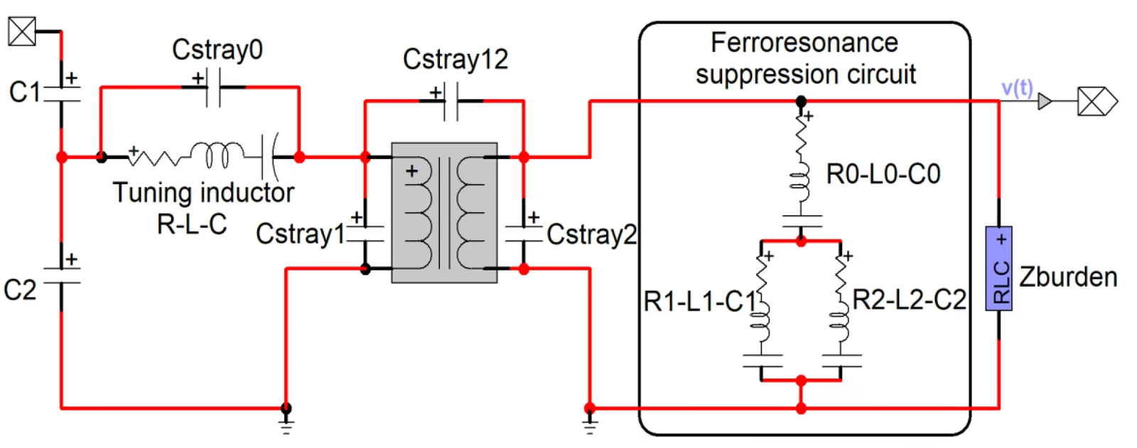
The EMTP® CapacitiveVoltageTransformer (CVT) device is the clearest library example of capacitive fast-front modelling. Its subcircuit is a capacitive divider (\(C_{1}\) top, \(C_{2}\) bottom) feeding a tuning-inductor branch (\(R, L, C\)) and an intermediate VT with a nonlinear magnetising branch. The documentation states that the four explicit stray capacitances must be included when fast transients are studied — in particular when the propagation of travelling waves from the CVT primary to the secondary has to be simulated:

Table 3 — CVT stray capacitances and their locations.

Stray Capacitance	Location
\(C_{stray0}\)	tuning-inductor stray capacitance
\(C_{stray1}\)	winding-1-to-ground
\(C_{stray2}\)	winding-2-to-ground
\(C_{stray12}\)	winding-1-to-winding-2

It is precisely \(C_{stray12}\) (winding-1-to-winding-2) in series with \(C_{stray2}\) (winding-2-to-ground) that forms the capacitive divider carrying the fast front from the CVT primary to the secondary — the same \(C_{12}/(C_{12}+C_{2g})\) mechanism above, realised inside a real EMTP® device. Without these strays, the CVT model reverts to its power-frequency behaviour and cannot reproduce the steep transferred surge that drives relay-measurement errors during faults. This makes the CVT device a usable, validated template for how capacitive fast-front transfer is represented in EMTP®. (The CVT also carries an optional ferroresonance-suppression circuit; see the instrument transformer page.)

The CVT example is useful because it shows how capacitances can be represented explicitly in an EMTP® instrument-transformer device. It should not be read as a general replacement for a detailed high-frequency power-transformer winding model.

Practical model selection

In EMTP® studies, the high-frequency representation is built by adding suitable terminal capacitances, using frequency-dependent branches, or fitting a black-box terminal model where frequency-response data exists. Internal winding studies need a dedicated detailed winding model and often manufacturer data.

Table 4 — Recommended high-frequency transformer model by study objective.

Study Requirement	Recommended Approach
External terminal overvoltage only	Terminal capacitance to ground, surge impedance, or a black-box terminal model (in EMTP®, added at the bushing nodes)
Surge transfer between windings at terminals	Multi-terminal (MIMO) black-box model or a capacitance-coupled terminal model; the CVT device with strays is a validated template
Internal winding voltage distribution	Lumped-ladder, STL, MTL or a manufacturer-supported winding model
Inter-turn or inter-disc insulation stress	Detailed internal model with winding geometry (not a stock EMTP® library device)
Lightning surge interaction with the connected network	Terminal high-frequency transformer representation (capacitances / FDB at the terminals)
Fast-front switching with frequency-dependent damping	Include frequency-dependent resistance / losses where data is available

Damping is a primary input

In resonance-dominated studies — resonant TRV, cable- or GIS-transformer interaction, repetitive switching — the assumed damping is a first-order input, not a refinement. The same capacitances and inductances with too little damping overestimate the resonant peak and stretch the decay, while too much damping hides a real overvoltage. A model with credible capacitances but arbitrary or default damping can be wrong by a large margin; damping (frequency-dependent losses, dielectric and eddy-current losses) must be set from measured response or realistic loss data wherever the result is resonance-sensitive.

The selection rule mirrors the overview page: choose by the physical behaviour to be represented, not by the component name. Above ~6–10 kHz the BCTRAN/nameplate matrix is no longer sufficient on its own — add capacitances, fit an FDB to measured data, or move to a special internal winding model — and reserve the detailed MTL/ladder models for the cases where inter-turn insulation stress, not terminal behaviour, is the question.

Common modelling mistakes to avoid:

using a low-frequency transformer model for lightning surge studies;
assuming the transferred surge voltage follows the power-frequency turns ratio;
using a terminal model to assess inter-turn insulation stress;
ignoring winding capacitances in fast-front studies.

Minimum data to request for a high-frequency study

Transformer rating and vector group; winding arrangement and tap position.
Bushing and terminal capacitances; surge / effective capacitance or measured frequency-response data.
Terminal admittance (or impedance) matrix where available.
Voltage-transfer measurements or manufacturer-calculated transfer functions.
Grounding and neutral treatment.
Connected cable / GIS / busbar layout; surge-arrester location and characteristics.
The intended frequency range over which the model is to be valid.
For internal-stress studies, winding geometry and insulation detail — normally proprietary to the manufacturer.

In practice: use a terminal high-frequency model when the objective is external-network overvoltage or surge transfer at the terminals; use a detailed internal model only when winding voltage distribution or inter-turn stress is required. Standard low-frequency transformer models should not be used alone for high-frequency surge studies unless capacitances or frequency-dependent behaviour are added.

Ultimately, high-frequency transformer modelling is a data-driven problem: the model is only as good as the frequency-response data, capacitances and manufacturer information behind it. Bolting added capacitances onto a low-frequency model improves its asymptotic behaviour but does not by itself reproduce winding resonance, damping or the internal voltage distribution — so for critical studies, support the model with frequency-response measurements or manufacturer data, and be explicit about whether it is intended for terminal behaviour, voltage transfer, or internal insulation stress.

Part Three Reading now

High-Frequency Models

Terminal versus internal models; multi-conductor and single-phase transmission-line and ladder winding models; capacitive voltage transfer; and the EMTP® capacitance / Frequency-Dependent Branch route above the BCTRAN validity limit.

Series progress 3 of 5

Part Four

Power-Transformer Device Catalogue

A working catalogue of the EMTP® power-transformer library devices — the ideal unit and m-winding ideal unit, the 2- and 3-winding nameplate-input transformers, and the BCTRAN matrix model — with formulas, input data and limitations.