Electromagnetic Transient Studies

Transformer Modelling in EMTP® — Low-Frequency Models

No single transformer model is correct under all low-frequency conditions. This part develops the matrix, saturable, topology-based and hybrid approaches, the single- and three-phase representations, and the core/winding/loss sub-models — woven throughout with their EMTP® realisation in BCTRAN and the nameplate-input transformers.

Reading time ≈ 14 min · Part Two of the series

Low-frequency transformer models are used when the transformer’s behaviour is governed by leakage impedance, winding resistance, magnetising current, core saturation, residual flux and losses. They suit studies such as energisation, inrush current, ferroresonance, low-frequency resonance, harmonic interaction and most switching studies below the first winding resonance.

The overview page introduced the general transformer model classes (black-, white- and grey-box); this page focuses on how the low-frequency models are implemented and used in EMTP® studies.

Low-frequency transients — energisation and de-energisation, inrush, ferroresonance, harmonic interaction, capacitor/reactor switching, controller interactions, temporary overvoltages — are dominated by the magnetic behaviour of the core (nonlinear magnetisation, saturation, and sometimes hysteresis) together with the short-circuit (leakage) impedance and the winding and core losses. Capacitive coupling is normally negligible in this band (see the frequency-band table on the overview page), so the building blocks are resistances, leakage inductances, ideal-ratio elements, and one or more nonlinear magnetising branches. The frequency range of validity for standard low-frequency models extends from DC up to the first winding resonance — typically a few kilohertz; for the EMTP® matrix model this is often around 6–10 kHz before terminal capacitances or frequency-dependent elements need to be added. These higher-frequency modelling options are discussed in the high-frequency modelling page.

These models should not be used as detailed winding models for lightning or very-fast-front studies. At higher frequencies, winding capacitances, travelling-wave behaviour and frequency-dependent terminal response become dominant — those effects are addressed separately in the high-frequency modelling page.

Key takeaway

For low-frequency studies the key inputs are leakage impedance, winding resistance, the magnetising branch, the saturation curve, residual flux and losses.
BCTRAN is suitable for a matrix-based low-frequency model built from standard transformer test data.
Nameplate-input transformers are suitable when nonlinear magnetisation and initial flux need to be represented.
If saturation, ferroresonance or unbalanced excitation matters, treat the magnetising-branch location and the zero-sequence flux path carefully.

Quick rule. Reach for BCTRAN when you need a robust multi-winding linear matrix built straight from standard test data; reach for the nameplate-input transformer when the study is dominated by nonlinear magnetisation, residual flux, inrush or ferroresonance. When both matrix coupling and saturation matter, keep BCTRAN but attach the nonlinear magnetising branch externally, across the winding closest to the core.

No single low-frequency model is correct for every condition. Four broad categories are used, and EMTP® provides a library device for each route:

Table 1 — Low-frequency transformer model categories and their EMTP® implementation.

Model Type	Simple Meaning	Typical Use	Main Limitation	EMTP® Implementation
Matrix-based	Coupled impedance / admittance matrices $[R]$, $[L]$ from test data	General low-frequency and multi-winding studies	Linear; based on power-frequency data	BCTRAN → RL coupled multiphase
Saturable / star	Per-winding branch + star point + nonlinear magnetising branch	Energisation, inrush and saturation studies	Magnetising-branch location may not be physically exact	Nameplate-input transformers (non-ideal unit)
Topology / duality	Represents the magnetic structure of the transformer	Studies where core construction and zero-sequence flux matter	Requires more transformer design data	Topological / duality circuits
Hybrid	Physical structure + measured / fitted data	More accurate practical modelling when data is available	More complex to parameterise	Combination of the above

Section 1

The four categories

Matrix-based models. The transformer is described entirely by impedance or admittance matrices relating terminal voltages and currents. For a single-phase multi-winding unit the steady-state relation is

\[ V = Z\,I, \]

$V$: vector of terminal voltages
$I$: vector of terminal currents
$Z$: terminal impedance matrix

and the corresponding time-domain branch equation is

\[ v = R\,i + L\,\frac{di}{dt}. \]

$v,\,i$: branch voltage and current
$R$: resistance matrix
$L$: inductance matrix

When the magnetising current is small (or zero) the inductance matrix $L$ becomes ill-conditioned or singular, so the admittance (nodal) form is preferred:

\[ I = Y\,V, \qquad \frac{di}{dt} = L^{-1}v - L^{-1}R\,i . \]

$Y$: terminal admittance matrix ($Y=Z^{-1}$)
$L^{-1}$: inverse-inductance matrix
$v,\,i$: branch voltage and current
$R$: resistance matrix

The matrix elements are obtained from nameplate, short-circuit, and no-load (excitation) tests, and phase coupling is included directly. The limitation is that the matrices are linear and only strictly valid at the test frequency; the nonlinear core must be attached externally at the terminals, and where it is attached matters once the core saturates (the saturated inductance is small, so its location dominates the response). This is the BCTRAN route in EMTP®.

Saturable transformer component (star circuit). Each winding is represented by a series branch meeting at a common star point, with a magnetising branch and, for three-phase core-type units, an explicit zero-sequence magnetising branch. It is simple and practical, but the single magnetising inductance can be placed at a topologically incorrect location; when the core saturates and that inductance collapses to its air-core value, the misplacement produces wrong inrush and ferroresonance behaviour. This is why it must be used with care for energisation and ferroresonance, and why the EMTP® nameplate-input devices give explicit control of the nonlinear-branch position (winding-1 side) and of the air-core slope.

Topology / duality models. The physical magnetic structure is mapped to an equivalent electrical circuit using the principle of duality: windings become MMF (current) sources, leakage paths become linear reluctances, and core limbs and yokes become saturable reluctances. The dual then yields an electrical network in which every branch corresponds to a physical part, so the nonlinear core is automatically at the correct location. Such models naturally reproduce per-limb saturation, inter-phase magnetic coupling, the zero-sequence flux path, and the differences between 3-legged, 5-legged, and shell core types. The price is the need for design data not contained in standard factory tests.

Hybrid models. These combine a topologically correct core with matrix or measured terminal parameters — physically meaningful structure, plus frequency-dependent winding resistance, capacitances, and a nonlinear magnetisation fitted to measurements. They are the most general and accurate, and the most data-hungry.

Section 2

Single-phase transformer models

T-equivalent. The classical two-winding model places the magnetising branch between two series leakage branches:

\[ R_{H},\;L_{H}\;\;\text{(HV winding)}\qquad R_{L},\;L_{L}\;\;\text{(LV winding)}\qquad R_{m}\;\parallel\;L_{m}\;\;\text{(core)} . \]

$R_{H},L_{H}$: HV-winding resistance and leakage inductance
$R_{L},L_{L}$: LV-winding resistance and leakage inductance
$R_{m}\parallel L_{m}$: core-loss resistance in parallel with the magnetising inductance

$R_{H},R_{L}$ and $L_{H},L_{L}$ come from the short-circuit test, $R_{m}$ and $L_{m}$ from the no-load test. The model is familiar but not topologically rigorous: the short-circuit test fixes only the sum of the two leakage inductances, so the split between $L_{H}$ and $L_{L}$ is arbitrary. This arbitrariness is harmless in the linear region but becomes important once the core saturates, because the magnetising branch then sits between two leakages whose individual values were never measured.

PI-type model. A more physically meaningful single-phase model uses a central linear leakage inductance with two (possibly unequal) nonlinear magnetising branches, one toward each winding. By distributing the nonlinear element to both ends it represents saturation more correctly than the single-branch T-model.

Winding model. Each winding is a series resistance plus a leakage inductance derived from short-circuit tests. With concentric windings the inner winding (usually LV) has the smaller leakage and the outer (HV) the larger; again the division of leakage between windings only matters under saturation, and higher accuracy requires winding-construction detail.

Core model and saturation parameters. The magnetising branch is a nonlinear inductance (saturation) in parallel with a resistance (core losses). Saturation governs energisation, inrush, ferroresonance, over-excitation, fault recovery and low-frequency resonance. At energisation the total flux is the sum of the residual (remanent) flux and the forced flux; deep saturation gives large, distorted inrush currents. The saturation curve is fixed by:

the nominal flux (knee region);
the exciting current at nominal flux;
the saturated (air-core) slope of the $\lambda\!-\!i$ curve;
the zero-current intercept;
the correct location of the nonlinear branch.

For energisation and ferroresonance the saturation curve is one of the most important inputs. If the saturated (air-core) slope is unknown, carry out a sensitivity study — it strongly affects inrush current and ferroresonance behaviour.

Residual flux

Residual (remanent) flux is a key initial condition for energisation studies: different residual-flux assumptions can produce very different inrush currents. Unless reliable measured or manufacturer data is available, energisation studies should test more than one residual-flux case.

Energisation is not a single case. Inrush is highly sensitive not only to residual flux but also to the switching instant (point on wave), source strength, winding connection and neutral earthing. The worst combination of switching angle and remanence rarely coincides with any one deterministic run, so a single energisation simulation should not be reported as the worst case unless the switching angle and residual-flux state behind it have been justified — otherwise sweep switching angle and residual flux together.

In EMTP® the nonlinear inductance is entered as instantaneous current–flux point vectors $\texttt{ILnonl}$ / $\texttt{PhiLnonl}$ with an optional per-phase initial flux $\Phi_{0}$. The peak flux scales as

\[ \Phi_{\text{peak}} \;\propto\; \frac{\sqrt{2}\,V_{\text{peak}}}{2\pi f}, \]

$\Phi_{\text{peak}}$: peak core flux
$V_{\text{peak}}$: peak applied voltage
$f$: supply frequency

and the curve can be entered either as RMS open-circuit current–voltage points (converted internally to current–flux) or directly as instantaneous current–flux points.

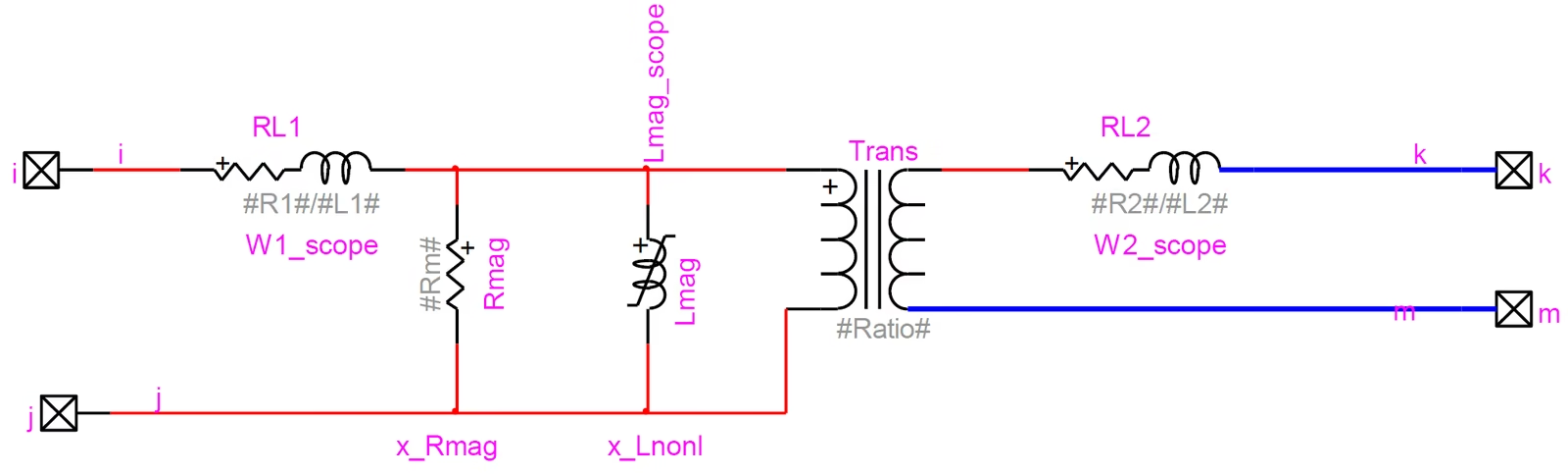
Single-phase non-ideal transformer building block — **Figure 1 —** Single-phase non-ideal building block.

Hysteresis and the three loss components. Real core losses are history-dependent and split into three parts: hysteresis, classical (eddy), and excess losses. For most low-frequency studies a single-valued (often two-slope piecewise-linear) saturation curve with a parallel loss resistance is sufficient. For ferroresonance, however, the loss representation is decisive: it provides the damping that determines whether the sustained oscillation decays or persists, so hysteresis and the full loss model matter there.

Treat damping as an input, not just an output. In ferroresonance and resonance studies the loss representation (core, winding, tank and the external circuit) is a deliberate modelling choice, not merely an active-power figure to check afterwards. The error cuts both ways: set it too low and the result is conservative but non-physical; set it too high and the excess damping can quietly hide a real risk. Where loss data is weak, bracket it from both sides rather than committing to one value.

RMS vs peak excitation data

Manufacturer excitation data is usually given as an RMS exciting current that lumps together the magnetising (reactive) and core-loss (resistive) currents. EMTP® nonlinear-inductance input needs an instantaneous current–flux relationship, so the two components must be separated and the RMS-to-peak conversion applied. Skipping this over- or under-states the knee and the loss.

Eddy currents in windings and core. Eddy currents are usually thought of as a loss mechanism, but in transient studies they also provide damping — reducing oscillations and reshaping the waveform — so they can matter in resonance, ferroresonance and switching studies. Changing flux induces eddy currents in two places:

In the windings: skin and proximity effects make the effective winding resistance frequency-dependent. This is represented by a Foster RL network fitted to the measured frequency response — a terminal model.
In the core: at higher frequency the flux is confined to a thin layer near the lamination surface, making both the magnetising inductance and the core-loss resistance frequency-dependent. This is captured with Foster or Cauer ladders; the Cauer form is more physical because its successive sections correspond to progressively deeper flux penetration. The number of sections grows with the frequency range to be covered.

Tank effect. During deep saturation, part of the flux may leave the core and pass through the tank or structural steel, which changes the apparent saturated inductance. Most practical low-frequency studies do not need a separate detailed tank model, but the tank effect should be kept in mind when selecting or estimating the saturation curve.

Matrix route in EMTP® — BCTRAN

In EMTP®, BCTRAN is best understood as a data-calculation function rather than just a transformer symbol: it converts standard transformer test data into coupled resistance and inductance matrices, which are then used by the coupled-multiphase RL representation.

BCTRAN is the data-calculation function that reproduces a three-phase, multi-winding transformer at power frequency from standard nameplate tests, producing coupled $[R]$ and $[L]$ (or $[R]$ and $[L^{-1}]$) matrices that are loaded into the RL coupled multiphase element. Its electrical data are entered on three tabs — Excitation data, Windings, and Short-circuit test data.

Magnetising / excitation. The positive- and zero-sequence shunt admittances $Y_{1}$ and $Y_{0}$ from the excitation tests are assembled into a 3×3 submatrix with self and mutual terms

\[ Y_{s}=\frac{Y_{0}+2\,Y_{1}}{3},\qquad Y_{m}=\frac{Y_{0}-Y_{1}}{3}. \]

$Y_{s}$: self (diagonal) shunt-admittance term
$Y_{m}$: mutual (off-diagonal) shunt-admittance term
$Y_{1}$: positive-sequence shunt admittance (excitation test)
$Y_{0}$: zero-sequence shunt admittance

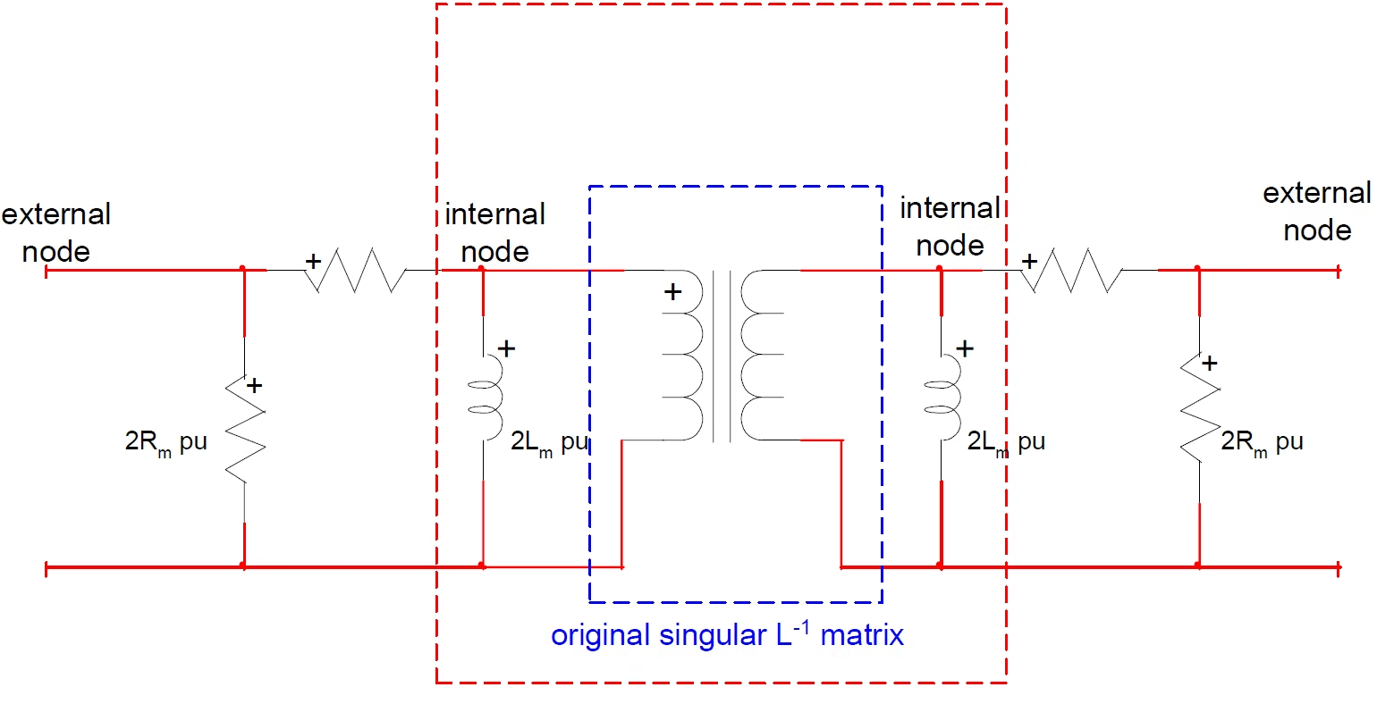
The imaginary parts (the magnetising inductances $L_{m}$) are folded into $[L^{-1}]$ to make it non-singular and invertible, while the loss resistances $R_{m}$ (hysteresis + eddy) are added as separate branches at the external nodes. The magnetising matrix may be connected across one winding, or $1/N$ of the pu value across all $N$ windings (on cylindrical windings it is best placed across the winding closest to the core).

Addition of magnetising branches in the BCTRAN model — **Figure 2 —** Addition of the magnetising branches in BCTRAN.

Short-circuit reactances. From each pairwise short-circuit test,

\[ X_{ik}=\sqrt{\,Z_{ik}^{2}-\bigl(R_{i}+R_{k}\bigr)^{2}\,}\quad\text{(pu)}, \]

$X_{ik}$: short-circuit (leakage) reactance between windings $i,k$ (pu)
$Z_{ik}$: measured short-circuit impedance between the two windings (pu)
$R_{i}+R_{k}$: combined pu load-loss resistance of the two windings

with $Z_{ik}$ the pu short-circuit impedance between windings $i,k$ and $R_{i}+R_{k}$ the pu load losses (or specified winding resistances) on the same MVA base. For closed-delta three-winding cases the equivalent-star relations

\[ X_{12}^{\text{closed}}=X_{1}+\frac{X_{2}X_{3}}{X_{2}+X_{3}},\qquad X_{13}=X_{1}+X_{3},\qquad X_{23}=X_{2}+X_{3} \]

$X_{1},X_{2},X_{3}$: equivalent-star branch reactances
$X_{12}^{\text{closed}},X_{13},X_{23}$: measured pairwise reactances (winding 3 a closed delta)

are solved for $X_{1},X_{2},X_{3}$ (resistances retained in the complex form), flagged by the DELTA parameter (Yyd and Ydd handled; Ddd is not). Winding resistances themselves can be derived from the load losses for $N=2$ or $3$ windings (assuming pu $R_{1}=R_{2}$ for two-winding); for $N\ge 4$ they must be supplied.

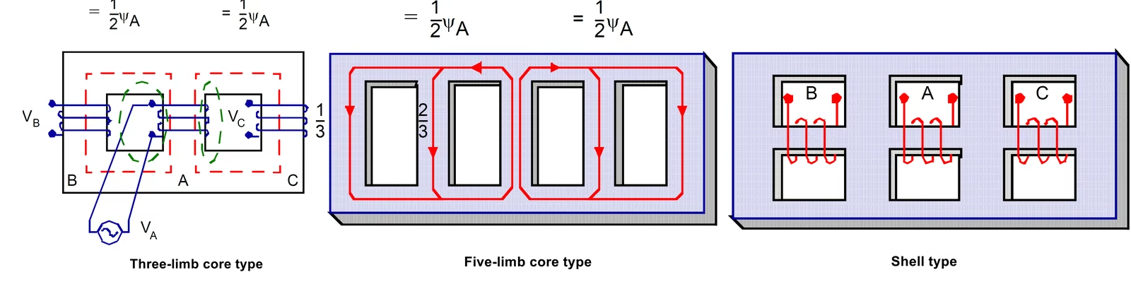
Zero-sequence excitation and core type. For a three-limb core the zero-sequence flux has no iron return path: exciting one phase (A) drives roughly half its flux back through phases B and C, inducing $V_{B}=V_{C}\approx -k\,V_{A}$. With $V_{A}=Z_{s}I_{A}$ and $V_{B}=V_{C}=Z_{m}I_{A}$,

\[ \frac{Z_{m}}{Z_{s}}=-\frac{Z_{\text{pos}}-Z_{\text{zero}}}{2Z_{\text{pos}}+Z_{\text{zero}}}=-k, \qquad \frac{I_{exc}^{0}}{I_{exc}^{+}}=\frac{1+k}{1-2k}. \]

$Z_{s},Z_{m}$: self and mutual zero-sequence excitation impedances
$Z_{\text{pos}},Z_{\text{zero}}$: positive- and zero-sequence impedances
$k$: coupling factor ($\to 0.5$ three-limb, $\approx 1/3$ five-limb/shell)
$I_{exc}^{0},I_{exc}^{+}$: zero- and positive-sequence exciting currents

For a 3-limb core $k\to0.5$ (the ratio diverges; a reasonable $I_{exc}^{0}\approx100\%$); for a 5-limb (or shell) core $k\approx1/3$, giving $I_{exc}^{0}/I_{exc}^{+}\approx4$. The zero-sequence excitation current must therefore not be ignored on three-limb cores. Closed deltas short-circuit the zero-sequence current, turning the zero-sequence excitation test into a short-circuit test (so the delta is opened for the test, and the zero-sequence excitation values become non-critical).

Three-limb, five-limb and shell core flux paths — **Figure 3 —** Core flux paths (three-limb, five-limb, shell).

Saturation (added externally). The nonlinear inductance is placed across the winding closest to the core (usually the tertiary). Its air-core slope is low — ≈ 2 × the short-circuit inductance — and the magnetising point already used in forming the matrix must be subtracted when defining the curve (e.g. if 0.03 % was used as the magnetising current for the impedance matrix, the 0.03 % point is subtracted from the nonlinear curve).

Numerical advantages over TRELEG. Because EMTP® uses a nodal-admittance formulation, BCTRAN allows an infinite magnetising impedance (a singular $[L^{-1}]$ is acceptable) and degenerates at DC to an uncoupled positive resistance matrix (the winding resistances) — better behaved than the older TRELEG. A floating (ungrounded) closed delta still gives undefined node voltages and a singular matrix; ground one terminal or add a small ground capacitance. Linear validity extends to ≈ 6–10 kHz; above that add winding-to-ground / inter-winding / inter-phase capacitances or use a Frequency-Dependent Branch (FDB) model. Autotransformers give reasonable results when treated as ordinary coupled windings; greater accuracy follows from re-casting the short-circuit data into the series/common sections (I, II, III).

Important modelling note

BCTRAN represents low-frequency transformer behaviour from standard test data. It does not automatically include winding capacitances or internal winding resonances. For studies above the low-kHz range, add winding-to-ground / inter-winding / inter-phase capacitances, a Frequency-Dependent Branch, or a high-frequency terminal/internal model — do not apply BCTRAN alone to fast-front or lightning studies.

Star / nameplate route in EMTP® — nameplate-input transformers

The EMTP® three-phase nameplate-input transformers (library Transformers.clf) are the topological/star realisation: three identical single-phase non-ideal units, one per phase, masked for nameplate data and per-phase initial flux. Each unit is

\[ \text{series } RL_{1} \;\rightarrow\; \bigl[\,L_{mag}\parallel R_{mag}\,\bigr]\;\rightarrow\; \text{ideal unit (Ratio)} \;\rightarrow\; \text{series } RL_{2} . \]

$RL_{1},RL_{2}$: primary- and secondary-side series leakage branches
$L_{mag}$: nonlinear magnetising inductance (saturation)
$R_{mag}$: core-loss resistance, parallel with $L_{mag}$
Ratio: ideal-unit turns ratio

Nameplate → parameters. The pu winding resistance and short-circuit impedance are

\[ R=\frac{P_{\text{loss}}}{S_{b}}\;\text{(pu)},\qquad Z_{sc}=\sqrt{X^{2}+R^{2}}\;\Rightarrow\; X\approx Z_{sc}\ \text{when } R\ll X . \]

$R$: pu winding resistance from the load-loss test
$P_{\text{loss}}$: load (copper) loss
$S_{b}$: rated (base) power
$Z_{sc}$: short-circuit impedance (pu)
$X$: leakage reactance (pu)

The leakage is split between windings by the ratio $D_{w}$:

\[ R_{1}=D_{w} R,\quad R_{2}=(1-D_{w})R,\quad X_{1}=D_{w} X,\quad X_{2}=(1-D_{w})X . \]

$D_{w}$: leakage-split ratio between the two windings
$R_{1},R_{2}$: primary- and secondary-side resistances
$X_{1},X_{2}$: primary- and secondary-side leakage reactances
$R,X$: total pu resistance and reactance

Base quantities.

\[ Z_{b1}=\frac{V_{b1}^{2}}{S_{b}},\qquad Z_{b2}=\frac{V_{b2}^{2}}{S_{b}},\qquad i_{b1}=\frac{1000\,S_{b}}{\sqrt{3}\,V_{b1}}\quad(\text{$S_{b}$ in MVA, $V_{b}$ in kV} \to \text{A}). \]

$Z_{b1},Z_{b2}$: base impedances of windings 1 and 2
$V_{b1},V_{b2}$: rated (base) voltages (kV)
$S_{b}$: rated power (MVA)
$i_{b1}$: base current of winding 1 (A)

Per-connection pu → ohm conversion uses connection factors $C_{1}$ (primary) and $C_{2}$ (secondary):

\[ R_{1}=C_{1} R\,Z_{b1}D_{w},\quad R_{2}=C_{2} R\,Z_{b2}(1-D_{w}),\quad X_{1}=C_{1} X\,Z_{b1}D_{w},\quad X_{2}=C_{2} X\,Z_{b2}(1-D_{w}), \]

$C_{1},C_{2}$: per-connection factors (primary, secondary)
$R,X$: pu resistance and reactance
$Z_{b1},Z_{b2}$: base impedances
$D_{w}$: leakage-split ratio

with the magnetising branch on the winding-1 side, $R_{m}=C_{1} R_{mag}Z_{b1}$:

Table 2 — Per-connection factors (C₁, C₂) and voltage ratio by winding connection.

Connection	$C_{1}$	$C_{2}$	Ratio
DD (Δ–Δ)	3	3	$V_{b2}/V_{b1}$
DY ±30 / DYg ±30 (Δ–Y)	3	1	$V_{b2}/(V_{b1}\sqrt{3})$
YD ±30 / YgD ±30 (Y–Δ)	1	3	$V_{b2}\sqrt{3}/V_{b1}$
YY / YgYg (Y–Y)	1	1	$V_{b2}/V_{b1}$

The flux and current point vectors are converted per connection. For the Δ-primary connections (DD, DY/DYg) the per-phase voltage is line-to-line, so

\[ \texttt{PhiLnonl}=\frac{1000\,\sqrt{2}\,V_{b1}}{2\pi f},\qquad \texttt{ILnonl}=\sqrt{2}\,\frac{i_{b1}}{3}\,i_{mag}, \]

$\texttt{PhiLnonl}$: flux point of the nonlinear-inductance curve
$\texttt{ILnonl}$: current point of the nonlinear-inductance curve
$V_{b1}$: base voltage; $f$ frequency; $i_{b1}$ base current
$i_{mag}$: per-unit magnetising current (Δ-primary scaling)

while the Y-primary connections (YD/YgD, YY/YgYg) divide the flux by $\sqrt{3}$ and use the full base current,

\[ \texttt{PhiLnonl}=\frac{1000\,\sqrt{2}\,V_{b1}}{2\pi f\,\sqrt{3}},\qquad \texttt{ILnonl}=\sqrt{2}\,i_{b1}\,i_{mag}. \]

$\texttt{PhiLnonl}$: flux point of the nonlinear-inductance curve
$\texttt{ILnonl}$: current point of the nonlinear-inductance curve
$V_{b1}$: base voltage; $f$ frequency; $i_{b1}$ base current
$i_{mag}$: per-unit magnetising current (Y-primary scaling, flux ÷√3)

Air-core inductance. The saturated-slope segment $L_{sat}$ — the winding inductance with the core fully saturated — is critical for energisation and ferroresonance and is usually missing from data sheets, because open-circuit tests reach only 110–115 % of nominal (enough for the elbow, not the air-core slope). Typical range 0.2–0.9 pu, default 0.3 pu; a sensitivity analysis is recommended. Per-phase initial flux $\Phi_{0a},\Phi_{0b},\Phi_{0c}$ is entered on the IC tab (otherwise taken automatically from steady state).

Modelling caution

Because the nameplate-input three-phase transformer is built from three independent single-phase units, it carries no common magnetic path between phases. This is fine for balanced positive-sequence studies, but it can mislead for zero-sequence excitation, single-pole switching, neutral displacement and unbalanced ferroresonance — especially on a three-limb core. For those, use a topology/duality or hybrid model whose core couples the phases.

Three-winding nameplate model

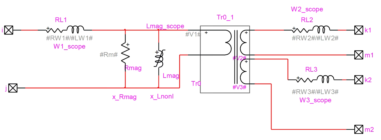
The single-phase building block gains a third series branch ($RL_{1},RL_{2},RL_{3}$), the magnetising branch $L_{mag}\parallel R_{mag}$ on winding 1, and an ideal three-winding unit with voltages $V_{1},V_{2},V_{3}$. The per-winding resistances follow from the three pairwise short-circuit tests via the equivalent-star conversion (shown here on a common MVA base; EMTP® first normalises each pair to its winding MVA $S_{b1},S_{b2},S_{b3}$ before forming the star, and negative leakages are possible and flagged):

\[ R_{1}=\tfrac12\bigl(R_{12}+R_{13}-R_{23}\bigr),\quad R_{2}=\tfrac12\bigl(R_{12}+R_{23}-R_{13}\bigr),\quad R_{3}=\tfrac12\bigl(R_{13}+R_{23}-R_{12}\bigr), \]

$R_{1},R_{2},R_{3}$: equivalent-star (per-winding) resistances
$R_{12},R_{13},R_{23}$: pairwise short-circuit-test resistances

each then scaled by the relevant impedance base $Z_{b}$ to ohms, with the inductances obtained cyclically from the reactances and $L=X/(2\pi f)$. The magnetising branch on winding 1 is $R_{m}=R_{mag}Z_{b1}$. The ideal-unit winding voltages depend on the connection. For YgYgD (grounded wye on windings 1 and 2, delta on winding 3),

\[ V_{1}=\frac{1000\,V_{b1}}{\sqrt{3}},\qquad V_{2}=\frac{1000\,V_{b2}}{\sqrt{3}},\qquad V_{3}=1000\,V_{b3}\ (\text{delta}), \]

$V_{1},V_{2},V_{3}$: ideal-unit winding voltages (YgYgD connection)
$V_{b1},V_{b2},V_{b3}$: rated winding voltages (kV)

whereas for YgDD (grounded wye on winding 1, delta on windings 2 and 3) both delta windings take the line-to-line value,

\[ V_{1}=\frac{1000\,V_{b1}}{\sqrt{3}},\qquad V_{2}=1000\,V_{b2}\ (\text{delta}),\qquad V_{3}=1000\,V_{b3}\ (\text{delta}), \]

$V_{1},V_{2},V_{3}$: ideal-unit winding voltages (YgDD connection)
$V_{b1},V_{b2},V_{b3}$: rated winding voltages (kV)

with the delta-winding star terms carrying the corresponding $\sqrt{3}$ / factor-3 scaling as in the two-winding case. Air-core segment, magnetisation input and initial-flux handling are identical to the two-winding nameplate model.

Three-winding non-ideal transformer building block — **Figure 4 —** Three-winding non-ideal building block.

Section 3

Three-phase transformer models

Three-phase low-frequency modelling is harder than single-phase because of the magnetic coupling through the common core and the strong dependence on core construction. Three model families parallel the categories above:

Matrix representation. Coupled $[R]$, $[L]$ (or $[L^{-1}]$) matrices computed from no-load and short-circuit tests — the BCTRAN route. Its advantages are the simplicity and the use of standard nameplate data (rated V/S, connection, short-circuit impedance, winding R, no-load current/losses, short-circuit losses); excitation losses enter as separate shunt resistances; winding resistances follow from short-circuit losses. It is linear and strictly power-frequency, so the nonlinear core is added externally (location matters), and the admittance formulation avoids the numerical problems of ignoring the excitation current.

Topology / duality. The physical magnetic structure is reproduced so that the zero-sequence flux path is correct for each core type:

3-legged (three-limb): zero-sequence flux must return through air, oil, tank and structure, giving a zero-sequence magnetising impedance very different from the positive-sequence value and a high zero-sequence exciting current (≈100 %, consistent with $k\to0.5$ above);
5-legged and shell: an iron return path of lower reluctance gives a much smaller difference ($k\approx1/3$, $I_{exc}^{0}/I_{exc}^{+}\approx4$).

Why core construction matters

For zero-sequence behaviour the core type is decisive. A three-limb core gives the zero-sequence flux no easy iron return path, so it returns through air, oil, tank and structure; five-limb and shell-form cores provide a lower-reluctance iron path. The same winding connection can therefore behave very differently depending on the core construction.

Duality-based models place the nonlinear core branch at the correct location and reproduce per-limb saturation and inter-phase coupling. This matters for single-phase switching, unbalanced faults, ferroresonance, energisation, zero-sequence overvoltages, over-excitation, neutral displacement, and unearthed / resonant-earthed neutrals. The limitations are tool-dependent equivalent circuits, parameter estimation from data not available in standard tests, and tank effects under unbalance/over-excitation.

Hybrid. A physically meaningful core topology populated with matrix or measured parameters, applicable across connections and extendable to nonlinear and frequency-dependent behaviour when data permit — more accurate, more complex.

Minimum data for a low-frequency model

Rated power and winding voltages;
vector group and phase shift;
winding resistances;
short-circuit (leakage) impedance on the correct MVA base;
no-load loss and excitation current;
the saturation curve — including the air-core slope, or a sensitivity range for it;
the residual-flux assumption;
tap position;
neutral-earthing arrangement;
core construction (3-limb / 5-limb / shell);
zero-sequence impedance or zero-sequence excitation data where unbalanced or earthing behaviour is in scope.

Selection. Choose by objective: an approximate terminal low-frequency response → matrix (BCTRAN); studies dominated by saturation, zero-sequence behaviour, or ferroresonance → topology or hybrid, or the nameplate-input devices with the nonlinear branch correctly placed and $L_{sat}$ supplied. For the device-level details of these EMTP® implementations see the Device Catalogue page; for the high-frequency extensions (terminal capacitances, FDB, internal winding models) see the High-Frequency Models page.

As a practical summary, the main low-frequency modelling routes map to study requirements as follows:

Table 3 — Recommended low-frequency transformer modelling approach by study requirement.

Study Requirement	Recommended Approach
Linear low-frequency multi-winding representation	BCTRAN / coupled multiphase RL model
Transformer energisation or inrush	Nameplate-input transformer with nonlinear magnetisation and initial flux
Ferroresonance	Nonlinear transformer with saturation, losses and relevant system capacitances
Zero-sequence or unbalanced behaviour	Model must reflect winding connection and core construction
Frequency-dependent damping	Add suitable frequency-dependent resistance / loss representation if data is available
High-frequency surge or lightning study	Use a high-frequency modelling approach, not a low-frequency model alone

Where this page ends. A low-frequency model returns a realistic inrush, voltage-recovery or ferroresonance response only if the nonlinear core, residual flux, losses, winding connection and zero-sequence path are all represented correctly. Once a transient carries significant energy above the first winding resonance, treat that model as only the base transformer representation: terminal capacitances, frequency-dependent branches, black-box terminal models or detailed winding models are then layered on top — the subject of the High-Frequency Models page.

In short. Low-frequency transformer modelling is a selection problem, not a data-entry exercise. The first decision is which physics dominates the study — linear leakage coupling, nonlinear saturation, residual flux, zero-sequence core behaviour or ferroresonance. BCTRAN, the nameplate-input transformers and the topology/hybrid models each answer a different part of that question, so match the model to the behaviour under investigation, supply the inputs that govern it (above all the saturation curve, air-core slope, residual flux and loss/damping), and confirm the frequency content stays below the first winding resonance — beyond that, hand over to the high-frequency representation.

Part Two Reading now

Low-Frequency Models

Matrix-based, saturable, topology and hybrid models; single- and three-phase representations; core saturation, hysteresis, eddy currents and tank — realised with EMTP® BCTRAN and the nameplate-input transformers.

Series progress 2 of 5

Part Three

High-Frequency Models

Terminal versus internal models; multi-conductor and single-phase transmission-line and ladder winding models; capacitive voltage transfer; and the EMTP® capacitance / Frequency-Dependent Branch route above the BCTRAN validity limit.

Connection	\(C_{1}\)	\(C_{2}\)	Ratio
DD (Δ–Δ)	3	3	\(V_{b2}/V_{b1}\)
DY ±30 / DYg ±30 (Δ–Y)	3	1	\(V_{b2}/(V_{b1}\sqrt{3})\)
YD ±30 / YgD ±30 (Y–Δ)	1	3	\(V_{b2}\sqrt{3}/V_{b1}\)
YY / YgYg (Y–Y)	1	1	\(V_{b2}/V_{b1}\)