This part is a working catalogue of the EMTP® power-transformer library devices: the lossless ideal units, the 2- and 3-winding nameplate-input transformers, and the BCTRAN matrix model. For each device it gives the concept, the equivalent circuit, the governing formulas, the input data, when to use it, and its limitations.
Reading time ≈ 17 min · Part Four of the series
This page links the transformer-modelling concepts from the previous sections to the transformer devices available in EMTP®. The aim is not only to describe each device, but to show when each is suitable, what data it needs, and which physical effects it does not represent.
Select a device using the modelling logic of the previous pages: low-frequency studies need leakage impedance, losses and magnetisation; high-frequency studies need capacitance and frequency-dependent behaviour; internal-insulation studies need detailed winding models beyond the standard terminal devices.
Read this as a catalogue, not a ranking: no single device is universally best — the right choice follows the study objective, so do not assume BCTRAN is always more accurate or a nameplate-input model always sufficient. Each device captures different physics.
This section is a working catalogue of the power-transformer library devices in EMTP® (the instrument transformers CT/VT/CVT are treated separately in the instrument transformer page). The devices fall into two families that map directly onto the model classes of the low-frequency modelling page:
Ideal units — lossless, stateless algebraic transformers used as building blocks and as ratio / level-shifting / power-amplifier elements (devices (a) and (b)).
Practical models — the nameplate-input transformers (devices (c) and (d)) follow the topological / star-circuit route, placing the nonlinear core branch on a defined winding; BCTRAN (device (e)) follows the matrix (admittance) route, producing coupled \([R]\) and \([L]\) (or \([R]\) and \([L^{-1}]\)) matrices for the RL coupled multiphase element. Both practical families are low-frequency models (valid to a few kHz — see the low-frequency modelling page and the validity note under BCTRAN).
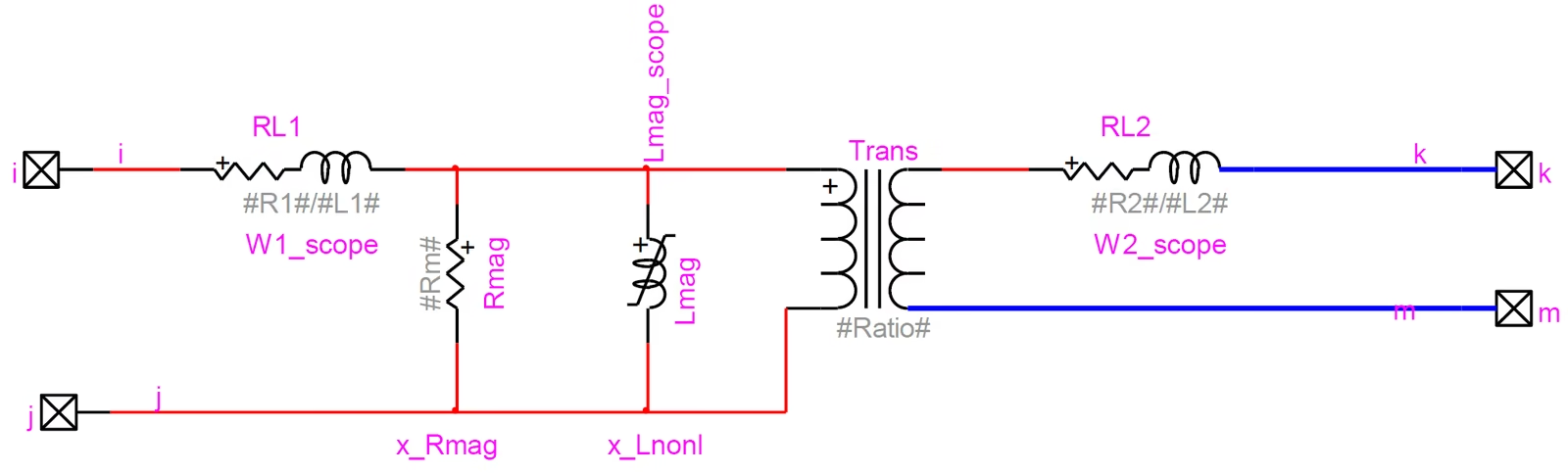
All nameplate and instrument transformers are masked subnetworks: one single-phase non-ideal unit (series RL → magnetising branch \([L_{mag}\parallel R_{mag}]\) → ideal unit → series RL) is replicated once per phase, and the mask scripts translate nameplate data into the primitive elements through the ModelData attribute. The nonlinear inductance is defined by the instantaneous current–flux point vectors ILnonl / PhiLnonl plus an optional initial flux \(\Phi_0\).
For each device below: concept/role, equivalent circuit, governing formulas, input data, when to use, and limitations. As a quick map, the table below summarises which EMTP® representation suits which study.
Table 1 — Practical comparison of EMTP® transformer devices and modelling approaches.
EMTP® Device / Approach
Typical Use
Main Represented Effects
Main Limitation
Ideal transformer
Voltage/current scaling without losses
Turns ratio only
No leakage, losses, saturation or capacitance
Multi-winding ideal transformer
Controlled ideal coupling between several windings
Ideal voltage/current transformation
Not for inrush, losses or fault-current limitation
Use a nameplate-input transformer (c/d) when nonlinear magnetisation, residual flux, inrush or ferroresonance dominate — you need a per-phase saturable core on a defined winding. Use BCTRAN (e) when you need a robust linear multi-winding, multi-phase coupled matrix from test data with correct interphase and zero-sequence coupling. When both matter, use BCTRAN with an externally connected nonlinear magnetising branch.
Section 1
(a) Ideal unit — 2-winding (Ideal_unit)
Concept / role. A pure, lossless ideal transformer with no internal state. Four 1-phase (General Signal) pins: winding 1 (primary) on pins \(i,j\); winding 2 (secondary) on pins \(k,m\). It is the elementary ratio element used inside the nameplate models and on its own for ideal level-shifting. The steady-state, load-flow, frequency-scan and time-domain models are all identical — the device is algebraic (no differential states).
Ideal transformer = a coupling device, not a transformer model
Use an ideal unit only when the transformer must transfer voltage and current by an ideal ratio. It does not represent leakage impedance, winding resistance, magnetising current, core saturation, inrush, losses, capacitances or internal resonances.
Governing formulas. With transformation ratio
\[ g=\frac{V_2}{V_1} \]
\(g\)
transformation (turns) ratio
\(V_1,V_2\)
primary and secondary rated voltages
(or entered directly as Ratio), the unknown is the winding-2 current \(i_{km}\) (from \(k\) to \(m\)). The voltage equation is
Input data. Primary voltage \(V_1\) and secondary voltage \(V_2\) (used to compute \(g\) when Ratio is not entered directly), orRatio \(=V_2/V_1\). Because the only transmitted datum is the ratio, variables may not be entered in the \(V_1\)/\(V_2\) fields. Pins cannot be deleted, and a pin's Phase attribute cannot be changed.
When to use. Ideal ratio change, base/voltage-level transitions, building-block role inside larger models, and any study where winding losses and magnetisation are deliberately excluded.
Limitations. No losses, no leakage, no magnetising branch, no saturation. Being a pure model, some configurations are mathematically impossible (e.g. shorting an ideal winding against an ideal source) and must be avoided; they yield singular or ill-posed network equations.
Do not use an ideal transformer when
inrush current is important; fault-current limitation by transformer impedance is important; losses are required; the voltage drop across the leakage impedance is required; core saturation or ferroresonance is being studied; or high-frequency capacitance or surge transfer is important. The same applies in TRV / recovery-voltage and insulation-coordination studies, where the missing leakage impedance, damping, saturation and capacitance change the result.
Section 2
(b) Ideal unit, m secondary windings (Ideal_unit_m-windings)
Concept / role. An ideal transformer with one primary and m secondary windings, each defining its own ratio \(g_n\) (secondary-n / primary). Beyond the multi-secondary ideal transformer, two extra operating modes turn it into a controllable system element: a Voltage-Controlled-Voltage-Source (VCVS) and a Power Amplifier. Ratios can be made controllable in the time domain via control signals.
Governing formulas — multiple secondaries. One voltage equation per secondary winding \(n=1\ldots m\):
\[ v_{k_n}-v_{m_n}-g_n\,v_i+g_n\,v_j=0, \]
\(v_{k_n},v_{m_n}\)
node voltages of secondary \(n\)
\(v_i,v_j\)
primary node voltages
\(g_n\)
ratio of secondary \(n\)
and the primary current is the gain-weighted sum of all secondary currents:
\[ i_{ij}=-\sum_{n=1}^{m} g_n\,i_{k_n m_n}. \]
\(i_{ij}\)
primary-port current
\(g_n\)
ratio of secondary \(n\)
\(i_{k_n m_n}\)
current of secondary \(n\)
\(m\)
number of secondary windings
For each secondary, \(i_{k_n}=i_{k_n m_n}\) and \(i_{m_n}=-i_{k_n m_n}\).
VCVS mode. The primary draws no current; the voltage equations are unchanged:
\[ i_{ij}=0. \]
\(i_{ij}\)
primary-port current — zero in VCVS mode, so the primary is a pure sensing port
The device then behaves as a voltage-controlled voltage source — the secondary ports impose voltages scaled by the ratios while the primary remains a pure sensing port.
Power-Amplifier mode. All port voltages are forced equal (\(v_{k_n}-v_{m_n}=v_i-v_j\)) and the primary current is multiplied by the gain. For a single port this gives
with \(v_{k_1 m_1}=v_{ij}\). Since voltage is preserved but current is multiplied by \(g\), power is amplified from the secondary port to the primary; with several secondary ports the primary power is the gain-weighted sum of the individual port powers.
Input data (Ratio tab). Number of secondary windings; primary winding voltage; one voltage per secondary winding (used only to compute the ratios \(g_n\)); checkboxes for Power Amplifier Mode, Voltage-Controlled-Voltage-Source Mode, Control all Ratios, and Control individual Ratios (winding numbers space-separated). A control-signal value of 0 preserves the previous/initial ratio of that winding. The Misc tab carries numerical options: Detect discontinuity due to a Ratio change (switches to Backward Euler at the discontinuity to avoid numerical oscillations, e.g. capacitor current on a sudden voltage change) and Resolve network equations after a Ratio change (applies the new ratio immediately, with no one-step control delay, when Simultaneous switching is on).
When to use. Multi-secondary ideal distribution; controllable on-load ratio changes in the time domain; VCVS as an ideal controlled source; power-amplifier idealisation in control/HIL-style diagrams.
Limitations. Lossless ideal model — same caveats as device (a). Inconsistent imposed conditions (e.g. connecting ideal voltage sources to amplifier ports on the secondary) make EMTP® take corrective actions that may not match the formulas above; avoid them.
Section 3
(c) Nameplate-input transformer, 2-winding — 3 separate 1-phase units (Three-phase_nameplate_input_transformers)
Concept / role. A practical three-phase transformer (library Transformers.clf) assembled from three identical single-phase non-ideal unit subnetworks — the standard building block of this section. Data are entered as nameplate quantities; the mask script converts them per connection type into the primitive RL branches, the magnetising branch, the ideal-unit ratio, and the nonlinear current–flux curve. Each phase can carry its own initial flux.
This is usually the most practical choice when standard transformer data is available and the study needs leakage impedance, winding losses, winding connection and nonlinear magnetisation. It suits many low-frequency transients — energisation, inrush and ferroresonance — provided the saturation curve and initial-flux assumptions are handled correctly.
Its accuracy depends strongly on the quality of the input data: rated voltage, rated power, short-circuit impedance, load losses, no-load losses, excitation current, winding connection, the saturation curve and the initial-flux assumptions should all be checked carefully.
Figure 1 — Single-phase non-ideal building block: series RL1 → magnetising branch \([L_{mag}\parallel R_{mag}]\) → ideal unit (Ratio) → series RL2.
Nameplate → per-unit parameters. Winding resistance from the load-loss test, and short-circuit reactance from the impedance test:
\[ Z_{b1}=\frac{V_{b1}^{2}}{S_b},\qquad Z_{b2}=\frac{V_{b2}^{2}}{S_b},\qquad i_{b1}=\frac{1000\,S_b}{\sqrt{3}\,V_{b1}}\ \text{(line-to-neutral, } S_b\text{ in MVA, } V_b\text{ in kV} \to \text{A)}. \]
\(Z_{b1},Z_{b2}\)
base impedances of windings 1 and 2
\(V_{b1},V_{b2}\)
rated (base) voltages (kV)
\(S_b\)
rated power (MVA)
\(i_{b1}\)
base current of winding 1 (A)
Per-unit and base quantities
Impedance, resistance and losses must be entered on the correct voltage and power base. Before entering data, confirm whether values are in ohms, per-unit or percentage, and whether they refer to winding voltage, line voltage or transformer rated power. A wrong base is one of the most common transformer-modelling errors.
Per-connection pu → ohm conversion uses connection factors \(C_1\) (primary) and \(C_2\) (secondary):
with the magnetising branch placed on the winding-1 side:
\[ R_m=C_1 R_{mag} Z_{b1}. \]
\(R_m\)
magnetising-branch (core-loss) resistance in ohms
\(C_1\)
primary connection factor
\(R_{mag}\)
pu core-loss resistance
\(Z_{b1}\)
winding-1 base impedance
Connection factors
Connection factors convert between the winding electrical quantities and the line quantities seen at the terminals; they depend on whether the winding is star, delta or another configuration. Wrong connection factors lead to wrong voltage ratios, impedance values or phase relationships — the connection type is not just a label.
The connection factors and ratio are:
Table 2 — Per-connection factors (C₁, C₂) and voltage ratio by winding connection.
Connection
\(C_1\)
\(C_2\)
Ratio
DD (Δ–Δ)
3
3
\(V_{b2}/V_{b1}\)
DY ±30 / DYg ±30 (Δ–Y)
3
1
\(V_{b2}/(V_{b1}\sqrt{3})\)
YD ±30 / YgD ±30 (Y–Δ)
1
3
\(V_{b2}\sqrt{3}/V_{b1}\)
YY / YgYg (Y–Y)
1
1
\(V_{b2}/V_{b1}\)
Magnetisation curve. Entered either as Current–Voltage (RMS open-circuit test points, converted internally to instantaneous current–flux) or directly as Current–Flux (instantaneous). For the DD connection the flux and current point vectors are scaled by
base voltage; \(f\) frequency; \(i_{b1}\) base current
\(i_{mag}\)
pu magnetising current (Δ-primary scaling)
For Y-primary connections (YD, YY) the flux vector carries an extra \(\sqrt{3}\) factor in the denominator and the current vector is \(\texttt{ILnonl}=\sqrt{2}\,i_{b1}\,i_{mag}\):
base voltage; \(f\) frequency; \(i_{b1}\) base current
\(i_{mag}\)
pu magnetising current (Y-primary scaling, flux ÷√3)
A similar transformation converts \(\Phi_{0a},\Phi_{0b},\Phi_{0c}\) into the per-phase initial flux \(\Phi_0\).
Air-core inductance \(L_{sat}\). An optional segment appended to the saturation curve, representing the winding inductance with the core fully saturated. Open-circuit tests typically reach only 110–115 % of nominal voltage — enough for the curve elbow but not the air-core slope, which is therefore often missing from data sheets. Typical range 0.2–0.9 pu, default 0.3 pu. It strongly affects energisation and ferroresonance results, so a sensitivity analysis is recommended.
Input data. Nominal power \(S_b\); frequency \(f\); winding voltages \(V_{b1},V_{b2}\) (RMS line-to-line); tap ratio; winding \(R\), \(X\) (pu or %); leakage-split ratio \(D_w\) (or explicit \(R_2,X_2\)); magnetisation data (current–voltage or current–flux); \(R_{mag}\); optional \(L_{sat}\); and on the IC tab the per-phase initial fluxes \(\Phi_{0a},\Phi_{0b},\Phi_{0c}\). Automatic initial conditions are otherwise taken from the steady-state solution.
When to use. General low-frequency three-phase studies that need a proper (non-ideal) core: energisation/inrush, ferroresonance, harmonic interaction, controller studies — wherever saturation and the correct ratio/connection handling matter but a full matrix or detailed HF model is not required.
Limitations. Low-frequency model (a few kHz); arbitrary leakage split via \(D_w\) (matters under deep saturation — see the low-frequency modelling page). Entering 0 for winding impedances forces ideal-network solving and may cause numerical instability. Data cannot be entered as variables (the mask is script-driven). Built from three independent single-phase units, so it does not represent the magnetic interphase coupling of a 3- or 5-limb core — use a topological/duality or BCTRAN model when zero-sequence core coupling is essential.
Section 4
(d) Nameplate-input transformer, 3-winding — 3 separate 1-phase units (Three-winding_nameplate_input_transformers)
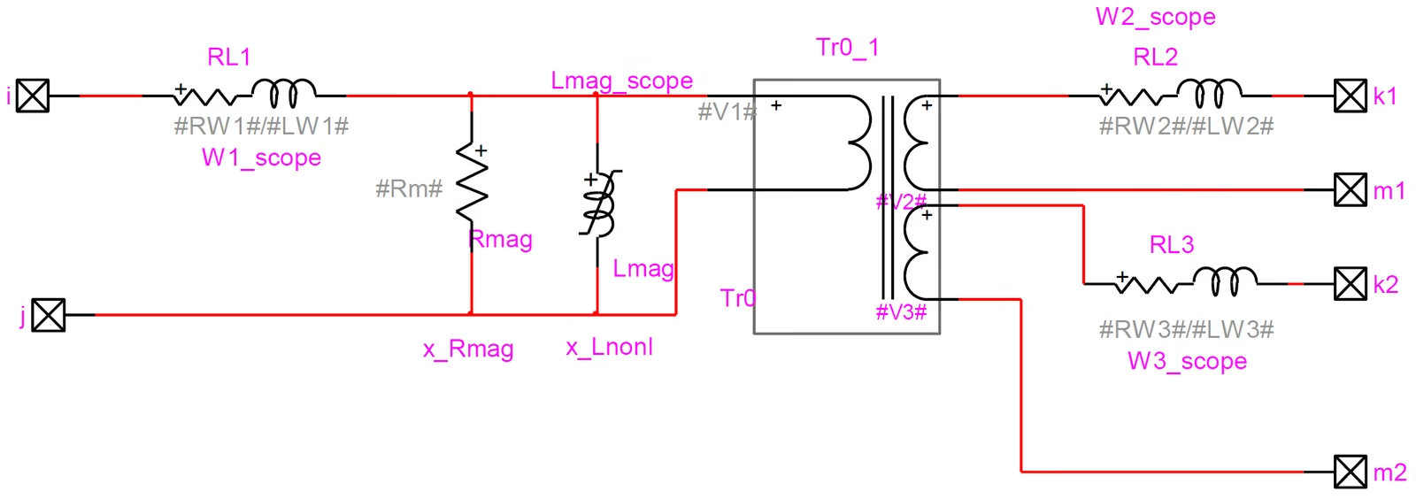
Concept / role. The three-winding extension of device (c), same construction philosophy. The single-phase building block now has three series RL branches (RL1, RL2, RL3), the magnetising branch \([L_{mag}\parallel R_{mag}]\) on winding 1, and an ideal 3-winding unit with winding voltages \(V_1,V_2,V_3\).
Three-winding modelling is not a simple extension of the two-winding case. The leakage impedances are normally specified between winding pairs, and these pairwise impedances must be converted into an equivalent-star representation. Depending on the test data, one equivalent leakage branch can become very small or even negative — this does not necessarily mean the data is wrong, but it must be checked carefully.
Figure 2 — Single-phase 3-winding building block (RL1, RL2, RL3 + magnetising branch on W1 + ideal 3-winding unit V1/V2/V3).
Equivalent-star parameters. The per-winding R and X are obtained from the three pairwise short-circuit tests (\(R_{12},R_{13},R_{23}\); \(X_{12},X_{13},X_{23}\)) via the equivalent-star transformation. Each pair is first normalised to its relevant winding MVA rating (\(S_{b1},S_{b2},S_{b3}\)) and referred to the common base \(S_{common}=S_{b1}\); writing the normalised terms, the star resistances are
(The per-pair MVA normalisation \(S_{common}/S_{b1}\), \(S_{common}/S_{b2}\), \(S_{common}/S_{b3}\) is applied to each term before forming the star; negative leakages are possible and are flagged.) The magnetising branch on winding 1 is
\[ R_m=R_{mag}\,Z_{b1}. \]
\(R_m\)
magnetising-branch resistance (on winding 1)
\(R_{mag}\)
pu core-loss resistance
\(Z_{b1}\)
winding-1 base impedance
Ideal-unit winding voltages. For the YgYgD connection (grounded-wye / grounded-wye / delta):
In both connections the nonlinear flux/current conversion uses the Y-primary forms \(\texttt{PhiLnonl}=1000\sqrt{2}\,V_{b1}/(2\pi f\sqrt{3})\) and \(\texttt{ILnonl}=\sqrt{2}\,i_{b1}\,i_{mag}\).
Available connections.YgYgD (Y–Y–Δ, grounded wye) and YgDD (Y–Δ–Δ, grounded wye); delta windings carry the \(\sqrt{3}\) connection factors as in the 2-winding case. A neutral pin appears if Y winding neutral is grounded is unchecked.
Input data. Frequency \(f\); winding voltages \(V_{b1},V_{b2},V_{b3}\) (RMS line-to-line); per-winding MVA ratings \(S_{b1},S_{b2},S_{b3}\); tap ratios (independent for windings 2 and 3); the pairwise R and X data (\(R_{12},R_{13},R_{23}\) / \(X_{12},X_{13},X_{23}\) when pu is used); magnetisation data; \(R_{mag}\); optional \(L_{sat}\) (same air-core treatment as (c)); and per-phase initial fluxes on the IC tab.
When to use. Three-winding low-frequency studies (e.g. autotransformer banks with a delta tertiary, three-winding generator step-up units) where the tertiary, the zero-sequence path through the delta, and saturation on the winding-1 core branch must all be represented.
Limitations. Same low-frequency, three-single-phase-unit limits as (c). The star transformation can yield negative leakage inductances (flagged); 0 winding impedances are not allowed, and the negative impedances that equations (6)–(11)/(18)–(23) may produce can make the case mathematically impossible or numerically unstable.
Concept / role. BCTRAN is not a placed transformer but a data-calculation function that converts standard nameplate test data into coupled matrices for the RL coupled multiphase element. It accurately reproduces the behaviour of a three-phase, multi-winding transformer at power frequency and is the matrix (admittance) counterpart to the topological nameplate models above. It outputs either \([R]\) and \([L]\) (reactance matrix in ohms at the stated frequency) or \([R]\) and \([L^{-1}]\) (inverse-inductance matrix in 1/mH, marked USE RB), loaded into the device through Load data from file.
Numerical advantages over TRELEG. BCTRAN allows infinite magnetising impedance — a singular \([L^{-1}]\) is acceptable because EMTP® uses a nodal-admittance formulation — and it degenerates to an uncoupled positive resistance matrix at DC (the winding resistances). TRELEG instead assumes finite magnetising impedance (and may produce an ill-conditioned model for large magnetising impedance) and degenerates to a coupled resistance matrix at DC that may or may not be stable. In general BCTRAN is better behaved than TRELEG.
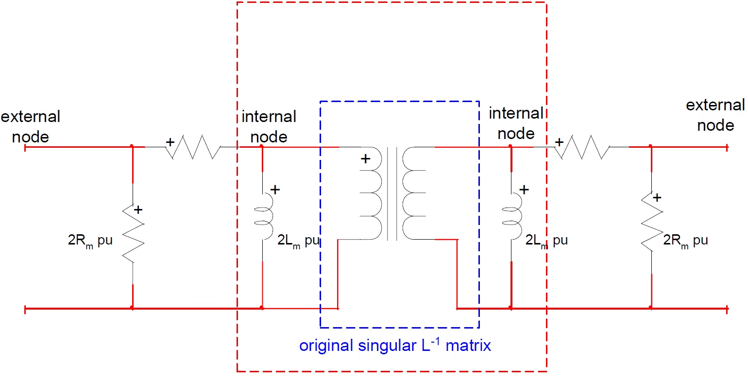
Figure 3 — Addition of magnetising branches across the windings (the dotted box shows the magnetising inductances folded into the \([L^{-1}]\) matrix; \(R_m\) added at the external nodes).
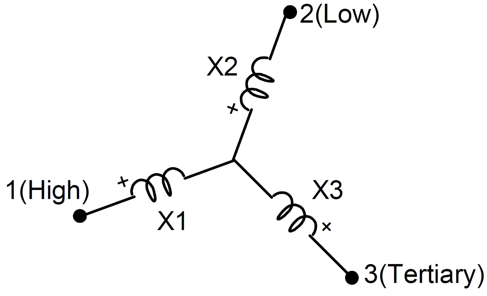
Figure 4 — Equivalent star circuit for the zero-sequence short-circuit tests of a three-winding transformer.
The three input tabs.
Excitation data — number of windings per core leg \(N\) (≤ 10); rated frequency; positive-sequence excitation test (\(I_{exc}^{+}\) in %, three-phase rating \(S^{+}_{rating}\), excitation loss in kW); zero-sequence excitation test (\(I_{exc}^{0}\), \(S^{0}_{rating}\), loss); single-phase-bank checkbox; Excitation test winding number; Magnetizing branch winding (if both numbers are unspecified, branches go across all windings; if the excitation test winding is specified, the magnetising branch winding must be too); and selection of which matrices to save.
Windings — rated \(V\) (line-to-ground for Y, line-to-line for Δ); winding resistance \(R\) (Ω/phase, average of the three phases); and the k-node / m-node reference names that appear on the RL-coupled-multiphase symbol (mandatory; GND denotes ground).
Short-circuit test data — per winding pair \((i,k)\): load loss \(P_{ik}\) (kW), positive-sequence impedance \(Z^{+}_{ik}\) (%) on \(S^{+}_{rating}\), zero-sequence impedance \(Z^{0}_{ik}\) (%) on \(S^{0}_{rating}\), and the DELTA and LOSS flags.
Magnetising / excitation submatrix. Positive- and zero-sequence shunt admittances \(Y_1,Y_0\) (from the excitation tests) form a 3×3 submatrix with self and mutual terms
The branch is connected either across one winding or, as \(1/N\) of the pu values, across all N windings. The imaginary parts (magnetising inductances \(L_m\)) are folded into the \([L^{-1}]\) matrix to make it non-singular and invertible; the loss resistances \(R_m\) (hysteresis + eddy) are added as separate branches at the external nodes. (The exciting current of 5-limb and single-phase units can often be ignored — the resulting singular \([L^{-1}]\) is harmless under the nodal formulation.)
Zero-sequence excitation (three-limb core). For a three-limb core the zero-sequence exciting current is high (≈ 100 %) and must not be ignored. Exciting phase A induces \(V_B=V_C\approx -k\,V_A\) in the other legs (about half of flux A returns through B and C); from \(V_A=Z_s I_A\) and \(V_B=V_C=Z_m I_A\),
For a three-limb core \(k\to 0.5\) (the limit gives infinite zero-sequence current; a reasonable \(I_{exc}^{0}\approx 100\%\), e.g. \(I_{exc}^{+}=0.5\%\) gives \(k=199/401\approx0.496\)). For a five-limb core \(k\approx\tfrac{1}{3}\Rightarrow I_{exc}^{0}/I_{exc}^{+}\approx 4\). A closed delta short-circuits the zero-sequence current, so the zero-sequence excitation test then behaves as a short-circuit test — the delta is assumed open for the test, and any reasonable \(I_{exc}^{0}\) (and \(S^{0}_{rating}\), loss) may be entered because the short-circuit data override it.
Winding resistance from load losses. For \(N=2\) or \(N=3\), \(R\) can be derived from the load losses (assuming pu \(R_1=R_2\) for two windings; three equations in \(R_1,R_2,R_3\) for three windings). For \(N>4\) the winding resistances must be supplied. The LOSS flag governs this: LOSS = 0 uses the supplied winding resistances; LOSS = 1 derives them from \(P_{ik}\), provided \(N\le 3\) and all \(P_{ik}>0\) (read-in resistances are then ignored).
where \(R_i+R_k\) are the pu load losses (or, if losses are not given, the specified winding resistances) on the same MVA base as \(Z_{ik}\). Equation \(X_{ik}\) is used for positive-sequence values and also for zero-sequence values when the zero-sequence test does not involve a third (delta) winding. For a three-winding closed-delta zero-sequence test the equivalent-star relations
are solved for \(X_1,X_2,X_3\) (resistances are retained in the full complex form of the closed-delta impedance). The DELTA flag marks an extra winding shorted in the zero-sequence test: DELTA = 0 (only windings \(i,k\) involved, e.g. all-wye grounded); DELTA > 0 = the number of the additional (delta) winding shorted in addition to winding \(k\). The program handles Yyd and Ydd connections but not Ddd with DELTA > 0. For a Ydd case where the test cannot be made between the two closed deltas, set \(Z^{0}_{ik}=0\) and the program estimates
estimated zero-sequence reactance between the two deltas
\(X^{+}_{d\text{-}d}\)
positive-sequence reactance between the deltas
\(Z^{0}_{y\text{-}2d},Z^{+}_{y\text{-}2d}\)
zero/positive-sequence impedance, wye to both deltas shorted
where "2d" denotes both deltas shorted in parallel.
Output matrices. Lower-triangular symmetric \([R]\)/\([L]\) (with a frequency header line, ohms) or \([R]\)/\([L^{-1}]\) (marked USE RB, 1/mH). The RL-coupled-multiphase device is then wired through the signals on its pins; the k-/m-node names are reference labels only.
Saturation — added externally. BCTRAN is linear; the nonlinear inductance is added across the terminals of the winding closest to the core (usually the tertiary in a three-winding unit) and sits in parallel with the unsaturated magnetising inductance. The air-core (saturated) slope of the \(\lambda\)–\(i\) curve is low — typically ≈ 2 × the short-circuit inductance. The magnetising current already used in forming the matrix must be subtracted when defining the nonlinear \(\lambda\)–\(i\) curve (e.g. if 0.03 % was used for the matrix, subtract 0.03 % from the saturation points).
BCTRAN in one line — linear unless you add a nonlinear branch
BCTRAN is a strictly linear coupled-winding model from short-circuit and open-circuit tests. On its own it has no nonlinear saturation, hysteresis, residual flux, winding capacitance or internal resonance. Where these matter, attach an external nonlinear magnetising branch across the winding nearest the core and justify its location physically — BCTRAN alone will not reproduce inrush, ferroresonance or remanence effects.
Floating delta. An ungrounded closed delta leaves the voltages-to-ground undefined → singular matrix and error termination. Fix by grounding one terminal or adding a small ground capacitance.
Frequency validity. Linear behaviour is reasonably accurate from very low frequency up to about 6–10 kHz. Above this, add capacitances (winding-to-ground, between windings, between phases) for the asymptotic response, or use a Frequency-Dependent Branch (FDB) model fitted to measured impedance-vs-frequency data (not available from standard factory tests — see the high-frequency modelling page).
Important modelling note
BCTRAN is mainly a low-frequency representation built from standard test data. It does not automatically include winding capacitances, internal winding resonances or detailed high-frequency surge behaviour. For fast-front studies, add capacitances, frequency-dependent elements or a dedicated high-frequency model.
Autotransformers. Treating the outer terminals as a normal transformer gives reasonably accurate results. Greater accuracy is obtained by re-casting the short-circuit data into the series/common sections — i.e. converting the H-L / H-T / L-T tests into I-II / I-III / II-III tests and representing the unit as three coupled windings I, II, III.
When to use. The preferred power-frequency route for accurate three-phase multi-winding matrix models from standard nameplate tests, especially where interphase coupling, zero-sequence behaviour (with a proper three-limb \(I_{exc}^{0}\)), and numerical robustness (infinite magnetising impedance) matter. Combine with an external nonlinear inductance for energisation/ferroresonance.
Limitations. Linear and power-frequency only (≲ 6–10 kHz); saturation is not built in and must be added externally on the correct winding; floating deltas must be grounded/capacitively tied; cannot handle Ddd with DELTA > 0; for \(N>4\) winding resistances must be supplied; HF accuracy requires added capacitances or an FDB model.
Summary — choosing among the power-transformer devices.
Table 3 — Summary of the EMTP® power-transformer devices and their primary use.
Device
Model Class
Core / Saturation
Phase Coupling
Primary Use
Ideal unit (a)
Ideal
none
none
Building block, ideal ratio
Ideal unit, m-windings (b)
Ideal
none
none
Multi-secondary, VCVS, power amp, controllable ratio
Nameplate 2-winding (c)
Topological / star
nonlinear on W1
none (3×1-ph)
LF 3-phase studies with saturation
Nameplate 3-winding (d)
Topological / star
nonlinear on W1
none (3×1-ph)
LF 3-winding (delta tertiary) with saturation
BCTRAN (e)
Matrix (admittance)
external, on winding nearest core
full matrix coupling
Power-frequency multi-winding matrix model
Instrument transformers (CT/VT/CVT), which reuse the same non-ideal-unit + nonlinear-core idea plus burden and divider/stray/FSC elements, are covered in the instrument transformer page.
Before you run the model — checklist
Rated voltage and power bases.
Winding connection and phase shift.
Leakage impedance and losses.
No-load current and no-load losses.
Saturation curve and air-core slope.
Initial flux / residual flux settings.
Neutral grounding and zero-sequence path.
Whether capacitances are required for the study.
Whether the model is valid for the frequency range of interest.
Common modelling mistakes to avoid:
using an ideal transformer where leakage impedance is required;
entering percentage impedance on the wrong base;
ignoring the phase shift of winding connections;
using BCTRAN for high-frequency surge studies without adding capacitances;
assuming a nameplate-input transformer automatically gives accurate inrush results without checking the saturation curve and residual flux.
What these standard devices do not give you
Out of the box, the ideal, nameplate-input and BCTRAN devices do not provide: (1) a validated high-frequency terminal admittance (impedance-vs-frequency) model; (2) voltage transfer to internal winding nodes; or (3) inter-turn / inter-disc insulation stress. For these, add winding-to-ground / inter-winding / inter-phase capacitances and frequency-dependent branches, fit a black-box / grey-box terminal model, or obtain a manufacturer-supported white-box winding model — see the high-frequency modelling page.
Specifying a manufacturer-supplied model. When an advanced terminal model is exchanged, agree the interface explicitly: terminal/node names, winding connections, voltage and current reference directions, grounding assumptions, units, the frequency range of validity, any external capacitances or bushings the model assumes, and — critically — whether it gives terminal admittance only or also voltage transfer to internal winding nodes. Terminal-admittance models are commonly exchanged in pole-residue or state-space form; a fitted model should have stable poles and be passive. No single model is best for every study, so state what each delivered model is valid for.
Manufacturer / customer model-exchange workflow. For procurement and detailed insulation studies the exchange is usually stepwise:
the manufacturer supplies a simplified terminal model for the system study;
the study engineer runs the network case and computes the overvoltage waveform at the transformer terminals;
that waveform is returned to the manufacturer;
the manufacturer applies it to a detailed internal design model to verify the winding stresses;
if needed, a more complete terminal or voltage-transfer model is requested.
This keeps the detailed winding design with the manufacturer while still validating internal stress against the real terminal transient.
In closing — match the device to the physics you need
Ideal units give ratio conversion only; nameplate-input transformers give a nonlinear low-frequency representation with connection handling and saturation on a defined winding; BCTRAN gives a robust linear coupled matrix with full interphase and zero-sequence coupling. High-frequency surge-transfer and internal-insulation studies fall outside all three and need added capacitances, fitted frequency-dependent models, or manufacturer-supported winding models. Pick the simplest device that still represents the effect you are studying.
Five-Part Technical Series
Transformer Modelling in EMTP®
A five-part guide to representing transformers in EMTP® — from the physical model-selection framework, through low- and high-frequency models, to the power-transformer device catalogue and the CT/VT/CVT instrument transformers.
04
04Part FourReading now
Power-Transformer Device Catalogue
A working catalogue of the EMTP® power-transformer library devices — the ideal unit and m-winding ideal unit, the 2- and 3-winding nameplate-input transformers, and the BCTRAN matrix model — with formulas, input data and limitations.