EMTP® Load Models

Types of Loads in EMTP®

A load is rarely just a number on a bus. EMTP® offers four practical load models — the PQ load (RLC), the PQ load with load-flow (LF), and the Variable static load in its individual and global forms. They are not interchangeable: they encode different engineering assumptions about load-flow participation, voltage and frequency sensitivity, and whether the distribution feeder is represented. This guide explains how each behaves, what it computes, and how to choose.

Reading time ≈ 24 min · EMTP® modelling guide

In a steady-state hand calculation a load can be just an active power \(P\) and a reactive power \(Q\). In an electromagnetic transient (EMT) study that is rarely enough, because EMTP® must turn the load into an actual circuit that the network solver can step through time. Depending on the model chosen, that circuit can be a fixed resistance, a parallel RLC equivalent, a series RL branch, a controlled current source, or a static load whose \(P\) and \(Q\) follow the bus voltage and the system frequency.

This is why several load models exist. The right one depends on whether the study cares about the load-flow operating point, steady-state initialisation, a frequency scan, voltage-dependent behaviour, frequency-dependent behaviour, or the distribution feeder between the bus and the real load.

Abbreviations used on this page

EMTP®Electromagnetic Transients Program

EMTPWorksThe graphical user interface used with EMTP®

PQActive- and reactive-power load

PActive power (W, kW, MW)

QReactive power (var, kvar, Mvar)

SApparent power (VA, kVA, MVA)

PFPower factor

RLCResistance, inductance and capacitance

LFLoad-flow

RMSRoot mean square

LLLine-to-line

puPer-unit

N pActive-power voltage exponent

N qReactive-power voltage exponent

K pActive-power frequency coefficient

K qReactive-power frequency coefficient

Y / YgWye / grounded-wye connection

DDelta connection

Key idea

PQ load (RLC) is a simple passive equivalent — fast and robust, but it does not participate in load-flow and is not voltage- or frequency-sensitive.
PQ load with LF participates in the load-flow solution and can start the transient from a realistic operating point, with voltage dependency through \(N_p\) and \(N_q\).
Variable static loads follow the exponential model — \(P\) and \(Q\) vary with voltage and frequency — for large-disturbance studies.
The global variant adds the distribution feeder impedance and shunt compensation; the individual variant does not.

Key terms used on this page

01Constant power

A load whose \(P\) (or \(Q\)) does not change with voltage — exponent \(N=0\).

02Constant current

Power varies approximately in proportion to voltage — exponent \(N=1\).

03Constant impedance

Power varies with voltage squared, like a fixed RLC — exponent \(N=2\).

04Exponential load model

The traditional static model expressing \(P\) and \(Q\) as powers of voltage with a frequency term.

05Load-flow participant

A load that imposes \(P\)/\(Q\) constraints in the load-flow solution, helping set the pre-disturbance operating point.

06Distribution feeder

The impedance between the upstream bus and the real load — transformers, cables and overhead lines.

07Shunt compensation

Capacitor banks or equivalent reactive support in the distribution substation.

08Aggregate load

A single equivalent representing the combined behaviour of many downstream loads.

09Controlled current source

A source adjusted each step so the load follows the exponential voltage/frequency law.

10Static vs dynamic load

Static loads follow algebraic V/f laws; dynamic loads (motors) add slip, stalling and recovery.

Section 1

Why the choice of load model matters

The four models represent different physical assumptions, so they can give materially different answers to the same study. The decision turns on a few questions: does the load need to participate in load-flow? Will the operating voltage differ much from nominal? Is voltage or frequency sensitivity important? Does the distribution feeder between the bus and the load need to be represented? And is the load even important to the result, or is it just background damping?

A useful mental model

A fixed RLC load obeys circuit laws — if the voltage drops, the current and power change naturally through the impedance. A voltage-dependent load instead uses equations to intentionally adjust \(P\) and \(Q\) with voltage magnitude. Constant-power behaviour draws more current as voltage falls; constant-impedance behaviour draws less. That difference can dominate a voltage-recovery result.

Section 2

The four load types at a glance

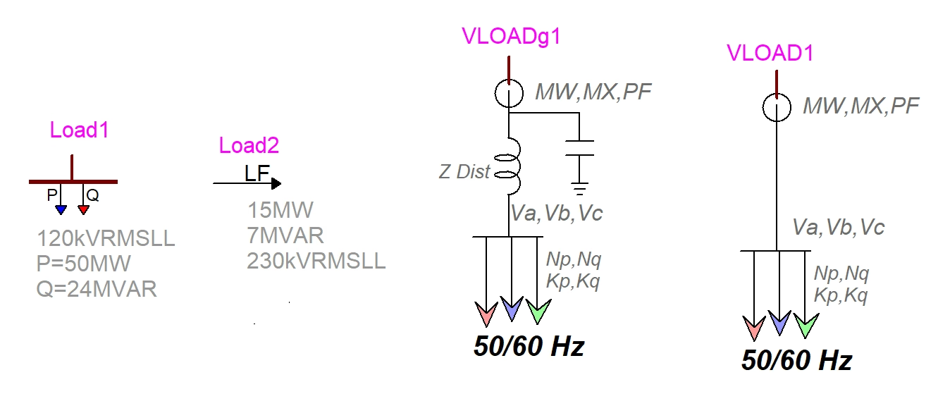
The four EMTP load models: Load1 a PQ load at 120 kV RMS line-to-line with P=50 MW and Q=24 Mvar; Load2 a PQ load with load-flow at 15 MW, 7 Mvar and 230 kV RMS line-to-line; VLOADg1 a Variable static load global form with MW, MX and PF inputs, a Z Dist series feeder impedance and a shunt capacitor; VLOAD1 a Variable static load individual form; both variable loads showing Va, Vb, Vc and Np, Nq, Kp, Kq at 50 or 60 Hz. — **Figure 1 —** The four EMTP® load models — the **PQ load** (Load1), the **PQ load with load-flow** (Load2, marked LF), and the **Variable static load** in its **global** form (VLOADg1, which adds the \(Z_\text{Dist}\) feeder impedance and a shunt-compensation branch) and **individual** form (VLOAD1). \(MW\), \(MX\) and \(PF\) set the nominal active power, reactive power and power factor; \(N_p, N_q\) set the voltage dependency and \(K_p, K_q\) the frequency dependency.

Fast selection rule

Need a correct load-flow / steady-state starting point? Use the PQ load with load-flow (LF). Just need a fixed \(P\) and \(Q\) with no load-flow constraint? Use the plain PQ load (RLC). Need the load to respond to voltage and frequency — or to bundle a distribution feeder and shunt compensation into one device? Use the Variable static load: the individual form for a load at a single bus, the global form when one device should also represent the feeder impedance and compensation.

Table 1 — The four EMTP® load models.

Load Type	Load-Flow?	Voltage Dep.?	Frequency Dep.?	Feeder Included?	Typical Use
PQ load (RLC)	No	No (once RLC)	No	No	Simple passive equivalent
PQ load with LF	Yes	Yes — via \(N_p,N_q\)	No	No	LF-initialised EMT studies
Variable Load individual	No standard LF role	Yes	Yes	No	Aggregate load on a modelled feeder
Variable Load global	No standard LF role	Yes	Yes	Yes	Substation aggregate load

Table 2 — Meaning of the voltage exponent \(N\) (applies to \(N_p\) for \(P\) and \(N_q\) for \(Q\)).

Exponent	Behaviour	Meaning
\(N=0\)	Constant power	Power does not change with voltage
\(N=1\)	Constant current	Power changes roughly in proportion to voltage
\(N=2\)	Constant impedance	Power changes roughly with voltage squared

Section 3

PQ load (RLC)

The PQ load (RLC) is the simplest model. It represents a three-phase load with equivalent R, L and C branches computed from the nominal voltage, active power and reactive power. The device is a masked subnetwork with a three-phase pin; the user enters the load nominal voltage \(V_\text{load}\) (RMS line-to-line), the total three-phase active power \(P\) and reactive power \(Q\) — or, optionally, apparent power \(S\) and power factor.

Scripted mask — no named variables

Because the mask is a scripted black box, you cannot enter undetermined named variables in the data fields. Data must be numeric (or accepted unit-based) values the mask can process — a common trap for newcomers who try to type a parameter name.

The active power is represented by a resistance, defined for positive power \(P>0\):

\[ R = \frac{V_\text{load}^2}{P} \]

\(R\): equivalent resistance
\(V_\text{load}\): load nominal voltage (RMS line-to-line)
\(P\): total three-phase active power

Voltage and power base must be consistent

The formula \(R = V^2/P\) is only correct when the voltage and power are on a consistent base. If \(V\) is the three-phase RMS line-to-line voltage, then \(P\) and \(Q\) must be the total three-phase powers. If the calculation is made per phase, use the phase-to-neutral voltage with per-phase \(P\) and \(Q\). Mixing line-to-line voltage with per-phase power is a common source of wrong R, L and C values.

Simple example

For a 50 MW, 24 Mvar load at 120 kV RMS line-to-line, using the total three-phase power and the line-to-line voltage consistently: \(R = 120^2/50 = 288\ \Omega\). The positive \(Q\) means the reactive branch is inductive, with \(X_L = 120^2/24 = 600\ \Omega\).

If \(P\le 0\) the resistance branch is automatically disconnected. The reactive power becomes an inductive branch for \(Q>0\) and a capacitive branch for \(Q<0\):

\[ X_L = \frac{V_\text{load}^2}{Q}\;(Q>0) \qquad L = \frac{X_L}{\omega} \qquad B_C = \frac{-Q}{V_\text{load}^2}\;(Q<0) \qquad C = \frac{B_C}{\omega} \]

\(X_L,\ L\): inductive reactance (\(\Omega\)) and inductance for an absorbed (inductive) \(Q\)
\(B_C,\ C\): capacitive susceptance (S) and capacitance for a generated (capacitive) \(Q\)
\(\omega,\ f\): angular frequency \(\omega = 2\pi f\) and system frequency

Positive \(Q\) is treated as an inductive load absorbing reactive power; negative \(Q\) is treated as capacitive reactive-power generation.

If \(Q=0\), both the inductive and capacitive branches are disconnected. A special rule: entering zero nominal voltage turns the device into a three-phase short circuit — never do this by accident. The same calculated R, L and C branches are used in the steady-state, frequency-scan and time-domain solutions.

The impedance does change with frequency in a frequency scan, because the branch reactances depend on frequency — but the model is still a passive RLC representation, not a behaviourally voltage- or frequency-sensitive load.

When to use it — and when not to

Use the PQ load (RLC) for a simple passive equivalent: basic switching transients, frequency-scan terminations, damping elements, training examples and any case where the load is not the focus and need not participate in load-flow. Avoid it when the load must participate in load-flow, when the operating voltage differs materially from nominal, or when voltage/frequency dependency, load recovery, or aggregate large-disturbance behaviour matter.

Don’t assume constant power

Once converted to RLC, the load does not hold constant \(P\) and \(Q\) during a transient — it behaves as an impedance. If you need constant-power behaviour during a disturbance, this is the wrong model.

Checklist before use

Is \(P\) positive? Is \(Q\) positive, negative or zero?
Is the entered voltage line-to-line RMS, and the power total three-phase?
Is the frequency correct, and the load intended to be passive / voltage-independent?
Are the resulting R, L and C values reasonable? (Voltage is not zero unless a short circuit is intended.)

Section 4

PQ load with load-flow (LF)

This model represents a one-phase or three-phase load (the three-phase version is a subcircuit of three one-phase devices) and can participate in the load-flow solution as well as steady-state, frequency-scan and time-domain. That load-flow participation is the key difference from the simple PQ load (RLC): it can be part of the solved operating point before the transient begins.

The user enters the nominal voltage \(V_\text{nominal}\), the nominal active and reactive powers \(P_\text{nominal}\) and \(Q_\text{nominal}\), the voltage exponents \(N_p\) and \(N_q\), and the data frequency. The exponents define how the load power follows the load-flow voltage:

\[ P_\text{specified}=P_\text{nominal}\left(\frac{V_\text{LF}}{V_\text{nominal}}\right)^{N_p} \qquad Q_\text{specified}=Q_\text{nominal}\left(\frac{V_\text{LF}}{V_\text{nominal}}\right)^{N_q} \]

\(V_\text{LF}\): actual voltage magnitude found by the load-flow solution (may differ from \(V_\text{nominal}\))
\(N_p,\ N_q\): voltage exponents (0 = constant power, 1 = constant current, 2 = constant impedance), used in both load-flow and steady-state
\(P_\text{specified}, Q_\text{specified}\): the powers imposed as load-flow constraints

For positive active power the parallel resistance is \(R=V_\text{load}^2/P\); for \(Q>0\) the inductance is \(L=V_\text{load}^2/(\omega Q)\); for \(Q<0\) the capacitance is \(C=-Q/(\omega V_\text{load}^2)\). When both \(P=0\) and \(Q=0\), the device becomes disconnected (infinite impedance) in all solutions. Where \(P\ge 0\) and \(Q>0\), an optional series-RL equivalent may be used instead of the parallel RLC, computed from:

\[ R + j\omega L = \frac{V_\text{load}^2}{P - jQ} \]

\(R + j\omega L\): series-RL equivalent impedance of the load
\(V_\text{load},\ P,\ Q\): the voltage and powers determined from the simulation options

Phase, connection and grounding options

One- or three-phase. Changing 3→1 retains phase-A quantities; changing 1→3 assumes balanced positive-sequence and copies phase-A into the other phases.
Positive-sequence input (three-phase): only phase-A data is entered, the load is assumed balanced, and phase-A is copied to the others — useful for balanced system-level studies.
Generic three-phase input with a Balanced option: unchecked allows different data per phase (for imbalance); checked copies phase-A to the others.
Connection: Wye (Y), grounded-wye (Yg) or Delta (D). Wye exposes the neutral pin; for Delta the entered powers are phase-to-phase values.
Show Ground Pin (one-phase): if not shown, the load is grounded automatically; if shown, it becomes ungrounded so extra series/grounding elements can be added.

Where the powers come from

In load-flow, \(P_\text{specified}\) and \(Q_\text{specified}\) become the constraints, and the device saves its voltages and currents to the load-flow solution file. In steady-state, if Retrieve Load-Flow solution data is checked (and a saved file exists with Start from Load-Flow solution on), the solved \(V_\text{LF}\) feeds the exponent equations to find \(P\)/\(Q\), and hence the R, L, C branches — so the time-domain run starts from a realistic operating point. If not retrieved, the nominal values are used (\(V_\text{load}=V_\text{nominal}\), \(P_\text{load}=P_\text{nominal}\), \(Q_\text{load}=Q_\text{nominal}\)). The frequency-scan and (un-initialised) time-domain models likewise default to nominal values.

Important caveat

The PQ load with LF is not a continuously controlled constant-power device during the time-domain run — its job is to set a correct load-flow / steady-state initial condition, after which the time-domain network sees an equivalent RLC representation that does not model frequency-sensitive or dynamic behaviour. In load-flow the device imposes \(P\) and \(Q\) at its bus, so if that bus is electrically isolated, EMTP® has no network path to supply the power and the constraints cannot be enforced — the load-flow will not converge.

Checklist before use

Will load-flow run before the time-domain simulation, and is Start from Load-Flow solution enabled?
Is Retrieve Load-Flow solution data required, and are \(N_p,\ N_q\) appropriate?
One- or three-phase? Balanced or per-phase? Y / Yg / D — and are powers total or phase values?
Is the device connected to the network before running load-flow (so it does not block convergence)?

Section 5

The variable static load

Static does not mean dynamic

The variable static load changes \(P\) and \(Q\) according to algebraic voltage and frequency equations. It does not model motor slip, motor stalling, thermal protection, contactor dropout, delayed recovery or composite-load dynamics. If those behaviours drive the study result, a motor or composite dynamic load model is required.

The variable static load implements the traditional exponential load model, expressed as a function of bus voltage magnitude and network frequency, with \(P\) and \(Q\) treated separately. Unlike a fixed RLC, it can change its active and reactive consumption as the voltage and frequency vary — the behaviour that matters in large-disturbance studies.

There are two versions, both masked subnetworks that can be unlocked to inspect or modify the internal design. The individual version models the load only; the global version also models the distribution feeder and shunt compensation. The model rests on the classic load-modelling literature (Price et al., IEEE 1988; Khodabakhchian et al., IEEE 1996; Kundur, Power System Stability and Control, 1993).

Section 6

Variable Load individual

The Variable Load individual device models the voltage- and frequency-dependent behaviour of a static aggregate load but does not include a distribution feeder — several of them can be hung off a feeder that is modelled separately. The three-phase load is built from three independent single-phase loads, each represented by a constant-impedance branch and a controlled current source adjusted to satisfy the exponential law:

\[ P = P_0\left(\frac{V}{V_0}\right)^{N_p}\left[\,1+K_p\left(\frac{f-f_0}{f_0}\right)\right] \]

\(P,\ P_0\): active power at the present and nominal conditions
\(V,\ V_0\): present and nominal voltage magnitude
\(N_p\): active-power voltage exponent
\(K_p\): active-power frequency multiplier
\(f,\ f_0\): measured and nominal frequency

\[ Q = Q_0\left(\frac{V}{V_0}\right)^{N_q}\left[\,1+K_q\left(\frac{f-f_0}{f_0}\right)\right] \]

\(Q,\ Q_0\): reactive power at the present and nominal conditions
\(N_q\): reactive-power voltage exponent
\(K_q\): reactive-power frequency multiplier

How to read \(K_p\) and \(K_q\)

\(K_p\) and \(K_q\) define how active and reactive power change when frequency moves away from nominal. A positive coefficient means the corresponding power increases when frequency increases; a negative coefficient means it decreases when frequency increases (so a negative \(K_q\), as in Table 4, means reactive demand falls as frequency rises). These coefficients should not be guessed — use project data, utility guidance or justified literature values.

The exponents set the load nature (0 / 1 / 2 = constant power / current / impedance), and the multipliers \(K_p\), \(K_q\) set the frequency sensitivity. The parallel constant-impedance branch is defined from nominal quantities, with multipliers \(n_R\) and \(n_X\) inside the expressions:

\[ R_0 = n_R\,\frac{V_0^2}{P_0} \qquad\qquad X_0 = n_X\,\frac{V_0^2}{Q_0} \]

\(R_0,\ X_0\): parallel constant-impedance resistance and reactance (subscript 0 = nominal)
\(n_R,\ n_X\): constant-resistance and constant-inductance multipliers

The multipliers \(n_R\) and \(n_X\) scale the constant-impedance branch. With \(n_R = 1\) the branch carries the full nominal active power (a pure-resistance load, e.g. incandescent lighting); larger values raise the branch impedance, so it carries a smaller share of the load while the controlled current source supplies the voltage- and frequency-dependent remainder. The multiplier therefore sits in the numerator — this matches the EMTP® documentation, where \(R_0 = n_R\,V_0^2/P_0\).

The controlled current sources live in a Current_inject subcircuit with a parameterised initialisation branch that switches off after a startup time of about \(0.1\ \text{ms}\) to support stable initialisation.

Low-voltage protection: \(K_\text{c\_IMP}\)

The parameter \(K_\text{c\_IMP}\) sets the voltage ratio below which the model reverts to constant-impedance behaviour. This matters for realism and numerical stability: a pure constant-power load at very low voltage would demand enormous current, which is unphysical and can destabilise the simulation. Switching to constant impedance below a threshold (typically \(0.5\)–\(0.7\) pu) avoids that.

Parameters

Table 3 — Variable Load individual parameters (typical ranges from the EMTP® documentation).

Parameter	Meaning	Units / Range
\(V_\text{nom}\)	Nominal bus voltage	kV RMS LL
Freq	Nominal frequency	Hz
\(n_R\)	Constant-resistance multiplier	1 to 10
\(n_X\)	Constant-inductance multiplier	1 to 5
\(MW_a\)	Nominal active power, phase a (same for b, c)	W (or MW)
\(MX_a\)	Nominal reactive power, phase a (same for b, c)	var (or Mvar)
\(N_p,\ N_q\)	Active / reactive voltage exponents	0–2 typical
\(K_p,\ K_q\)	Active / reactive frequency multipliers	—
\(K_\text{c\_IMP}\)	Voltage ratio below which constant impedance applies	0.5 to 0.7

A note on the names: the EMTP® mask calls these \(MW_a\) and \(MX_a\). \(MW_a\) is the nominal active power for phase A and \(MX_a\) is the nominal reactive power for phase A — not a reactance \(X\). Enter the value in the unit the mask expects (for example W/MW or var/Mvar via the unit suffix).

Typical exponent values

The EMTP® documentation gives representative values for common load classes — a useful starting point when project-specific data are unavailable:

Table 4 — Typical values for common loads (from the EMTP® variable-static-load documentation).

Load	\(N_p\)	\(N_q\)	\(K_p\)	\(K_q\)	\(n_R\)	\(n_X\)
Fluorescent lighting	1.0	3.0	1	−2.8	10	2
Incandescent lighting	1.56	0	0	0	1	10
Colour TV	2.0	4.8	0	−4.6	4	2
Substation load — winter (Canada)	1.4	2.0	1	−1	2	2
Substation load — summer (Canada)	1.0	3.0	1	−1	4	2

Default scopes let you validate behaviour during the run: measured frequency, total \(P\) and \(Q\), power factor, the per-unit phase voltages, and the controlled-current-source amplitude (used to check model stability).

When to use it — and when not to

Use the individual variable load when voltage and/or frequency sensitivity matters and the feeder is modelled separately — voltage-dip studies, frequency-disturbance studies and other large-disturbance EMT simulations where a fixed RLC is too simple. Avoid it when a simple passive load suffices, when load-flow participation is required, when the feeder must be inside the same model (use the global version), when detailed motor dynamics are needed, or when you have no defensible values for \(N_p,\ N_q,\ K_p,\ K_q\).

Section 7

Variable Load global

The global version is the individual exponential load plus a representation of the distribution feeder impedance, distribution-transformer equivalent and shunt compensation. That makes it the natural choice for an aggregate substation load, because real loads connect through transformers, cables, feeders and compensation — not directly to the transmission bus.

Table 5 — Additional Variable Load global parameters.

Parameter	Meaning	Units / Typical Range
\(\text{Perc\_ZDist}\)	Distribution impedance on the load-MVA base	pu
\(\text{Ratio\_XR}\)	X/R ratio of the distribution feeders	2 to 5
\(\text{Ratio\_Comp}\)	Ratio of compensator capacitance to substation load MVA	0.1 to 0.3
\(\text{Ratio\_MVA\_Dis}\)	Distribution-transformer MVA to load MW ratio	1.3 to 2.0
\(\text{Iron\_Dis\_XFO}\)	Distribution-transformer iron-loss percentage	0.3% to 0.6%

The distribution impedance represents the voltage drop between the upstream bus and the actual load, so the load-terminal voltage differs from the bus voltage — which shapes load voltage, current, reactive demand, voltage recovery, fault contribution and damping. The X/R ratio sets how inductive the feeder is, affecting voltage drop, damping, fault-current angle and transient response. The shunt compensation (via \(\text{Ratio\_Comp}\)) can significantly influence reactive balance, voltage profile, resonance, recovery and frequency-scan behaviour.

Avoid double-counting

The global model already contains feeder impedance and compensation. Do not add external feeder impedance or compensation again, and do not use it together with an explicitly modelled distribution feeder unless that double-counting is intentional. Watch for resonance introduced by unrealistic compensation. For example, if a 5% distribution-feeder impedance is already represented by an external transformer/cable/feeder model, do not also enter the same 5% inside \(\text{Perc\_ZDist}\) — that would make the downstream load appear electrically farther away than it really is.

When to use it — and when not to

Use the global variable load for an aggregate substation/transmission-bus load where the feeder is not modelled explicitly but its impedance and compensation should be included, especially in large-disturbance and voltage-recovery studies. Avoid it when the distribution feeder is already modelled in detail, when a simple passive load is enough, when load-flow participation is the main requirement, when the feeder/compensation data cannot be reasonably assumed, or when dynamic motor behaviour dominates.

Section 8

Comparison of the four load types

Table 6 — Side-by-side comparison.

Feature	PQ (RLC)	PQ with LF	Var. Individual	Var. Global
Simple to use	Excellent	Good	Moderate	Harder
Load-flow participation	No	Yes	No standard LF role	No standard LF role
Time-domain use	Yes	Yes	Yes	Yes
Voltage dependency	No	Yes (\(N_p,N_q\))	Yes	Yes
Frequency dependency	No	No	Yes	Yes
Feeder included	No	No	No	Yes
Shunt compensation included	No	No	No	Yes
Best for LF-initialised EMT	No	Yes	No	No
Best for large-disturbance static load	No	Limited	Yes	Yes
Best for aggregate substation load	Limited	Possible	Possible	Best
Data required	Low	Medium	Medium	High
Risk of wrong assumptions	Low	Medium	Medium	High

Section 9

Selection guide by study type

Table 7 — Recommended load model by study.

Study	Recommended	Avoid
Simple switching transient	PQ load (RLC)	Variable global (unless V/f matters)
Load-flow initialised EMT	PQ load with LF	PQ (RLC) if LF consistency needed
Frequency scan	PQ (RLC) or PQ with LF	Nominal-only if feeder/comp. matters
Voltage-dip study	Var. individual (feeder modelled) / global (not)	Fixed RLC alone
Frequency-disturbance study	Variable individual / global	PQ (RLC) and PQ with LF
Transmission-level aggregate load	Variable global	—
Detailed distribution feeder	Var. individual on the modelled feeder	Variable global (double-count)
Load not important	PQ load (RLC)	—

Section 10

Common mistakes

Common load-modelling mistakes

Using PQ load (RLC) when the EMT run must start from a solved load-flow operating point — use PQ with LF instead.
Assuming a PQ load stays constant power in the time domain — once converted it behaves as an impedance.
Confusing voltage-dependent static behaviour with dynamic behaviour — these models have no motor slip, stalling or recovery.
Using Variable Load global while also modelling the feeder separately — double-counts feeder impedance.
Using arbitrary \(N_p,\ N_q,\ K_p,\ K_q\) without project data, literature or justified assumptions.
Ignoring low-voltage behaviour — check the \(K_\text{c\_IMP}\) constant-impedance threshold.
Ignoring connection type — Y, Yg and D differ, especially in unbalanced studies.
Misreading the \(Q\) sign — positive \(Q\) is inductive, negative \(Q\) is capacitive.
Forgetting the per-phase vs total three-phase power convention (and Delta phase-to-phase values).
Forgetting that zero \(P\) and \(Q\) disconnects the PQ-with-LF device.

Section 11

A practical decision path

Need load-flow participation? → use PQ load with LF. Otherwise continue.
Is a simple passive RLC equivalent enough? → use PQ load (RLC). Otherwise continue.
Need voltage and frequency dependency? → use a variable static load. If not, choose PQ (RLC) or PQ with LF by initialisation need.
Is the distribution feeder modelled explicitly? → Variable Load individual. If not, and feeder/compensation should be included → Variable Load global.
Is dynamic motor behaviour important? → these static models may be insufficient; consider a motor or composite dynamic load model.

What to document

Always record the selected model with its voltage base, power base, connection type, voltage exponents \(N_p,\ N_q\), frequency coefficients \(K_p,\ K_q\), the constant-impedance threshold, any feeder/compensation assumptions, and whether the run started from load-flow. Suggested report wording, for example for the global model:

Example report wording

“The load was represented using the EMTP® Variable Load global model to capture an aggregate substation load including voltage and frequency sensitivity, distribution-feeder impedance and shunt compensation, because the detailed downstream distribution feeder was not explicitly modelled.”

Key message

Choose the load model from the study objective, not convenience. Use PQ load (RLC) for a simple passive equivalent, PQ load with LF when the load must participate in load-flow and set a correct pre-disturbance operating point, Variable Load individual when voltage/frequency dependency matters and the feeder is modelled separately, and Variable Load global when the feeder and shunt compensation should sit inside the aggregate load. The most common error is using a simple PQ/RLC load where load behaviour actually drives the result — fine for non-critical switching, but not for voltage dips, frequency excursions or aggregate substation studies.

Types of Loads in EMTP®

Why the choice of load model matters

The four load types at a glance

PQ load (RLC)

When to use it — and when not to

Checklist before use

PQ load with load-flow (LF)

Phase, connection and grounding options

Where the powers come from

Checklist before use

The variable static load

Variable Load individual

Parameters

Typical exponent values

When to use it — and when not to

Variable Load global

When to use it — and when not to

Comparison of the four load types

Selection guide by study type

Common mistakes

A practical decision path

What to document

Henry Gras

Simple technical notes for power system studies